Appointment scheduling for blood donors in combination with walk in donors

University of Twente

Faculty of Electrical Engineering,

Mathematics & Computer Science

Master Thesis

Appointment scheduling for blood donors in

combination with walk-in donors

Author:

Marieke Dijkink

Supervisors:

Prof. dr. N.M. van Dijk

S.P.J. van Brummelen, MSc

Abstract

Contents

1

Introduction . . . .

3

1.1

Motivation of research . . . .

3

1.2

Thesis Outline . . . .

3

2

Literature review . . . .

4

2.1

Appointment scheduling . . . .

4

2.2

Blood donation . . . .

4

2.3

Waiting time models . . . .

4

3

The blood donation process . . . .

6

4

Analysis of arrival patterns and service time distribution . . . .

7

4.1

Arrival patterns . . . .

7

4.2

Service time distribution . . . .

8

5

Waiting time models . . . 10

5.1

Network of non-preemptive M/M/c queues with priorities . . . 10

5.2

Network of M/M/1 queues with capacity reservation . . . 11

6

Schedule model . . . 12

6.1

Heuristic to generate schedules . . . 12

6.2

Rating schedules . . . 15

6.3

Heuristic to determine schedule . . . 17

7

Simulation models . . . 19

7.1

First simulation model . . . 19

7.2

Second simulation model . . . 20

7.3

Determining number of runs . . . 22

8

Results . . . 23

8.1

Comparing waiting time models section 5.1 and 5.2 . . . 23

8.2

Simulation model 1 . . . 24

8.3

Simulation model 2 . . . 24

8.4

Schedules with dierent penalty functions . . . 27

9

Conclusion and Recommendations . . . 29

9.1

Conclusion . . . 29

9.2

Recommendation . . . 30

0.5

. . . 38

0.6

. . . 39

0.7

. . . 40

0.8

. . . 41

0.9

. . . 42

0.10

. . . 43

0.11

. . . 44

0.12

. . . 45

0.13

. . . 46

0.14

. . . 47

0.15

. . . 48

B Arrival patterns analysis xed locations

49

1 Introduction

1.1 Motivation of research

Sanquin is a company that takes care of blood donation to full the demand for blood products. To collect blood

Sanquin has xed and mobile locations. At most xed location plasma and whole blood donation can be done.

At mobile locations only whole blood donations can be done. Plasma donors always come with an appointment.

Whole blood donors come on walk-in basis. A whole blood donor is invited to donate, within a certain time frame

the donor can decide if he/she comes and when.

In the near future there will be an online appointment system, such that whole blood donors can make an

appoint-ment. Sanquin decided which part of the agenda will be open for a donor. Within this period the donor is free to

choose a day and time. To come without appointment will remain possible. The aim is to have 80% of appointments,

the remaining 20% will come on walk-in basis. To stimulate whole blood donors to make an appointment, whole

blood donors with appointment will get priority over whole blood donors without appointment. Plasma donors

already have priority over whole blood donors, this will stay the same in the future.

The aim of this resource is to determine which appointment possibilities, slots, should be open for donors to make

an appointment. For blood donors it is important that the waiting time at the blood donation location is low.

So waiting should be taken into account. There has to paid attention to the possibility of no-shows. Further the

targets, number of blood donation per week needed, should be met. The percentage of no-shows is known for each

location. Depending on this percentage, it is determined how many donors should be asked to donate to meet the

targets.

1.2 Thesis Outline

In this thesis the focus will be on appointment scheduling for whole blood donors, taking into account the waiting

time a donor has to face at the donation location. In section 2 a review will be given of the available literature on

appointment scheduling for blood donation. This will extended with some literature on appointment scheduling in

health care and some literature of waiting time distributions for more general queues. For the current situation with

100% walk-in donors the arrival patterns are analysed in section 4. In the same section also service time distributions

are tted using the service time data. One of the queueing models from literature is used to evaluate waiting time

for the blood donation system. This non-preemptive

M/M/c

queueing model with priorities is explained in section

5. In the same section another queueing model to evaluate waiting time is explained, this model uses

M/M/

1

2 Literature review

Appointment systems are applied in many areas of healthcare. Those appointment systems can take into account

scheduled/unscheduled arrivals, patients with priorities, no-shows and punctuality of the patients. All of these

elements are also needed for a appointment system at blood collection sites. Therefore, this section has been split

into three parts. First, in section 2.1, attention is paid to some articles about appointment systems in healthcare.

Then, in section 2.2, the focus will be on the literature around scheduling appointments for blood donation. Finally,

in section 2.3, the literature of two waiting time models that can be used for modelling waiting time for blood donors

will be discussed. The second waiting time model is used in this thesis and will be explained more in section 5.1.

2.1 Appointment scheduling

Appointment scheduling for the blood donation process has rarely been discussed in literature, but in a broader

healthcare setting it is quite extensively studied. In (1) a review of literature is given on appointment scheduling

in outpatient clinics.

The more basic models consider one type of patients, who only have to go to one service point (e.g. a doctor) and

have an appointment (e.g. (2)). These basic models are extended with the possibility of no-shows (e.g. (3, 4, 5)) and

punctuality of patients (e.g. (4, 6)). In (7, 8) a combination of scheduled and unscheduled patients are considered.

Further in (7, 8, 9) patients with dierent priorities are handled.

In (10) appointment scheduling is done with a model considering two time periods. Included, a time scale for

appointment planning (long term) and one for the service process during the day (short term). This way, both

the arrivals of scheduled and unscheduled patients can be taken into account. The dierent time scales give the

possibility to measure access time, time between making the appointment and having the appointment, and waiting

time during the day. No-shows are also taken into account.

2.2 Blood donation

To plan appointments, insight in the arrival patterns of blood donor is required. In (11, 12, 13, 14) these arrival

patterns are studied. In (11) data mining is used, while in (12) logistic regression is used. In (13, 14) the arrival

patterns are studied by analysing the patterns visually.

A few papers use simulation to study the blood collection site (13, 14, 15, 16, 17). The simulation models are

made to study and improve the current donation process. In (14) also an LP model is used for determining the

minimal number of sta members needed to handle the arriving donors and satisfy the waiting time norm. With

these simulation models most existing literature about simulation models for the blood donation system is covered.

Waiting time is an important performance metric for blood collection sites. To keep blood donors satised the

waiting time should be as low as possible. In (18) a waiting time model is derived for whole blood donors coming

on walk-in basis.

Analytic models to schedule blood donors are introduced in (19, 20). These are the only analytic scheduling models

in the literature of blood donation. In (19, 20) the models consists of scheduled arrivals and walk-in arrivals.

Further they have a stability condition, the workload should always be smaller than one. All donor types have the

same priority. The models takes into account no-shows. In (19) an mixed integer non linear programming (MINLP)

model is used to schedule donors and reduce waiting time. The blood donation process is modelled as an open

Jackson network. An approximation of total waiting of donors arriving at a phase of the donation process in a time

interval is used. In (20) a multi-criteria mixed integer programming (MIP) model is used to schedule donors and

reduce waiting time and overtime (working after opening hours).

this way a donor of a lower class can have a higher priority than higher class donor. If a server nishes a service,

it starts serving the patient that has accumulated the most "priority points" since its arrival. This means that a

lower priority class patient does not have to wait until all higher class patients are served, waiting time gives a

lower class patient more priority. The waiting time distribution is given via the LST (Laplace-Stieltjes transform)

of the waiting time distribution. The accumulating priority system is method used for blood donation. At a blood

donation location for plasma and whole blood donation, plasma donors have priority over whole blood donors. So

normally a plasma donors will be rst to get service. Sometimes, if a whole blood donor has to wait really long,

a sta member handles a whole blood donor rst. In (23) there is a common service rate, they treat a

M/M/c

queue. In the articles (24, 25) the service time is exponentially distributed and the average service duration is class

dependent, which can be denoted as an

M/M

/c

queue. Only in the article (22) a general service time distribution

is discussed with a class dependent service rate, but they limit to one queue (

M/G

/

1

).

Another way to model the blood collection process is by using a general priority queue. In the articles (26, 27, 28, 29)

the multi-class non-preemptive M/M/c queue is discussed, in (30) the multi-class non-preemptive M/G/1 queue.

In (26, 27, 30) the waiting time is calculated via the LST of the waiting time distribution. The waiting time density

function and waiting time probability distribution are derived in (28). To calculate the waiting time distribution

elementary lattice paths counting is used. The LST corresponding to the derived waiting time distribution is

calculated to show it coincides with the one derived in (27). In (29) the probability function from (28) is specied

for two classical priority queues, the non-preemptive

M/M/c

queue with equal service rates and the non-preemptive

3 The blood donation process

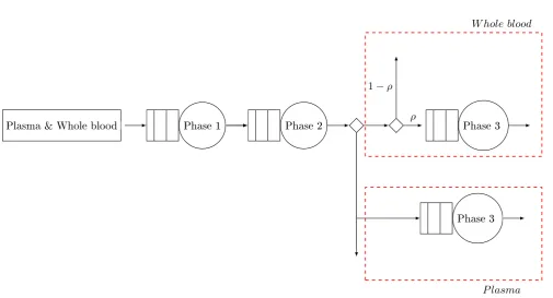
In this section the blood donation process will be explained. Two types of blood donation are considered, whole

blood donation and plasma donation. The focus is on whole blood donation, since appointment scheduling for whole

blood donors is done in this thesis. The donation processes of whole blood and plasma donation are partly mixed,

therefore also plasma donation will play a part. Both types of donors enter the building and start in the waiting

area of the registration. The donors stand in line, until the sta member at the registration desk is available. The

donor will be registered and gets a questionnaire. Between the registration desk and the medical check there is a

area where donors can sit down to ll in the questionnaire. After the questionnaire is lled in the donor goes to

the waiting area of the medical check. At the medical check area there are several rooms. A donors enters one of

the rooms and a sta member will do some tests and goes through the lled in questionnaire. To donate blood

the donation has to be safe for the donor and the recipient. The donated blood has to full certain criteria. On

the questionnaire there are questions to get this information. If the donor does not pass the medical check then

a donor is deferred. Depending on the situation a donor is invited to come back when the blood donation criteria

can be met or the donor must end his/her donation career. If a donor passes the medical check then the donor

can go to the donation area. There are some chairs to sit down while waiting on a bed. At the donation area are

beds with donation equipment besides them. Part of the beds can be used for plasma donation, the remainder can

only be used for whole blood donation. When a bed is available the donor can lie down. The rst available sta

member will connect the donation equipment and the donation starts. After a certain amount of blood/plasma is

donated, the machine will be uncoupled. The donor can go to the canteen area to have something to drink and

eat before going home. This to make sure the donor is al right The registration and medical check is the same

for whole blood donors and plasma donors, both types use the same resources. At the donation the two types are

separated, because more equipment is required for plasma donation. The whole donation process is shown in gure 1.

Plasma & Whole blood

Phase 1

Phase 2

Phase 3

W hole blood

Phase 3

P lasma

ρ

1

−

ρ

4 Analysis of arrival patterns and service time distribution

In this chapter an analysis of the arrival patterns of donors and the service time is discussed. This analysis is done

with data from 2015 of all xed locations in the Netherlands. This data is from the ocial database of Sanquin.

4.1 Arrival patterns

As the situation is now, whole blood donor come on walk-in basis. This makes the arrival process uncertain. As

already explained in section 1.1, in the near future there will be plasma donors and whole blood donors with and

without appointment. To get a good mix of these three donor types, the arrival pattern of whole blood donors in

the current situation (only walk in) will be analysed.

As explained in section 3 each blood donation location has certain sessions at which the location open. Arrival

patterns are analysed per location. At each location (almost) all days of the same type have the same session.

The type of day is Monday, Tuesday, Wednesday, Thursday or Friday. Therefore rst will be studied if the arrival

patterns are similar for all days of the same type. To statistically check if two arrival patterns are the same,

so if they come from the same continuous distribution, the two-sample Kolmogorov-Smirnov test is used. The

null hypothesis is that the data in vectors

x

and

y

come from the same continuous distribution, the alternative

hypothesis that the data come from dierent continuous distributions. If the null hypothesis is not rejected the

two-sample Kolmogorov-Smirnov test returns the test decision 0, otherwise 1. Per location all days of the same

type are compared, so if there are N type

r

days then the results can be put in a NxN matrix, say A. For example

at entry (n,m), with

1

≤

n, m

≤

N

, of matrix A, there is the test result of a type

r

day number n compared to

a type

r

day number m. Per type

r

day it is calculated what percentage of a type

r

days is not the same as the

type

r

day considered. This is calculated with equation 1a. The results can be put in a Nx1 matrix, say B. For

example at entry (n,1) of matrix B, there is the percentage of type

r

days not the same as type

r

day number n.

The smaller the percentages in B, the more likely that the arrival patterns of days of type

r

are similar for the

location considered.

B

(

i,

1) =

PN

j=1

A

(

i, j

)

N

·

100%

∀

i

= 1

, ...,

49

(1a)

PN

i=1

1

(

B

(

i,

1)

>

0

.

1)

N

·

100%

(1b)

To decide if the arrival patterns of days of type

r

can be considered the same, the percentage of rates bigger than

0.1 in matrix B is calculated with (1b). If the percentage determined with (1b) is smaller than 15% the arrival

patters of days of type

r

are considered to be the same. For 91% of the xed locations the arrival patterns of days

of the same type (and the with the same session) can be considered the same with this denition. This means that

it is reasonable to conclude that days of the same type (with the same session) have similar arrival patterns.

The next step is to compare days with the same session. So if a day of type

r

1

and a day of type

r

2

(same location

and

r

1

6

=

r

2

) have the opening hours 8.00-11.00, study if the arrival patterns of those days are the same. This

is done for the locations with where the arrival patterns of days of the same type are the same. If for example

the arrival patterns of day type

r

1

are the same, but the arrival patterns of day type

r

2

are not the same then

this location is not considered. Again the two-sample Kolmogorov-Smirnov test is used. If the arrival patterns

belonging to days of type

r

1

are compared to arrival patterns belonging to days of type

r

2

, then all days of type

r

1

are compared to all days of type

r

2

. If there are

N

days of type

r

1

and

M

days of type

r

2

, then the results can

be put in a

N xM

and a

M xN

matrix, say H1 and H2. For example at entry (n,m) of H1, with

1

≤

n

≤

N

and

1

≤

m

≤

M

, there is the test result of day number n of type

r

1

compared day number m of type

r

2

.Per day of

type

r

1

the percentage of days of type

r

2

not the same as that one day of type

r

1

is calculated, this is done with

equation 2a. Also per day of type

r

2

the percentage of days of type

r

1

not the same as that one day of type

r

2

is

calculated, this is done with equation 2b. If a day of type

r

1

is similar to all days of type

r

2

, then the percentage

of days of type

r

2

not similar to that day of type

r

1

is small. The result can be put in a

(

N

)

x

1

matrix, say G1. If

a day of type

r

2

is similar to all days of type

r

1

, then the percentage of days of type

r

1

not similar to that day of

type

r

1

is small. The result can be put in a

(

M

)

x

1

matrix, say G2.The smaller the percentages in G1 or G2, the

G

1(

i,

1) =

PM

j=1

H

1(

i, j

)

M

·

100%

∀

i

= 1

, ..., N

(2a)

G

2(

i,

1) =

PN

j=1

H

2(

i, j

)

N

·

100%

∀

i

= 1

, ..., M

(2b)

PN

i=1

1

(

G

1(

i,

1)

>

0

.

1)

N

·

100%

(2c)

PM

i=1

1

(

G

2(

i,

1)

>

0

.

1)

M

·

100%

(2d)

To decide if the arrival patterns of days of type

r

1

can be considered the same as the arrival patterns of days

of type

r

2

with the same session, the percentage of rates bigger than 0.1 in matrix G1/G2 is calculated with

(2c)/(2d). The arrival patters of days of type

r

1

are considered to be the same as the arrival patters of days of

type

r

2

, if both percentages, determined with (2c) and (2d), are smaller than 15%. For 90% of the xed locations

that are considered the arrival patterns of dierent type days, but the same session can be considered to be similar

with this denition. This means that it is reasonable to conclude that dierent type days, but with the same

session, have similar arrival patterns.

Last step is to analyse if days with dierent sessions have similar arrival patterns. The method is the same

as for comparing days with the same session. Now days with dierent sessions are compared. For 84% of the

xed locations that are considered the arrival patterns of dierent type days and with dierent sessions can be

considered to be not similar with this denition. Days of dierent type and with dierent sessions can have similar

arrival patterns if the opening hours could not be dened correctly. For examples sometimes one donor can come

outside opening hours, but this is not seen as outside opening hours. So this day gets assigned dierent opening

hours than there have been in practice. Concluding it is reasonable to conclude that dierent type days and with

dierent session, do not have similar arrival patterns.

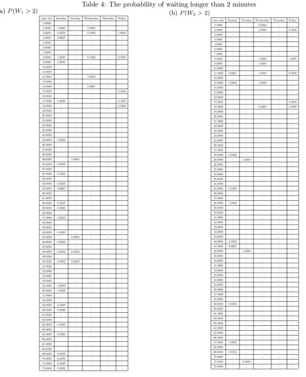
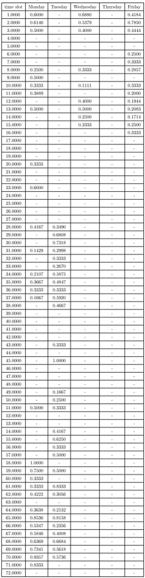
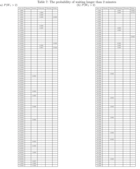
Both analyses are done for all locations and all day types. In appendix B, the B, G1 and G2 matrices are shown for

all blood donation locations. The matrices are ordered per location. The opening times of each location are shown

in appendix C.

4.2 Service time distribution

The next step is to analyse the service time of donors. The blood donation process consists of three phases,

as explained in section 3. For each of these phases a tting distribution for the service time has to be found.

These distribution are needed later in section 5 for the waiting time models and for the simulation models in

section 7. To compare dierent probability distribution the program/script ALLFITDIST, found on the website

of Mathworks, is used. With this program the following (continuous) probability distributions are tted to the

service time data: Beta, Birnbaum-Saunders, Exponential, Extreme value, Gamma, Generalized extreme value,

Generalized Pareto, Inverse Gaussian, Logistic, Log-logistic, Lognormal, Nakagami, Normal, Rayleigh, Rician, t

location-scale and Weibull. To nd out which distribution ts the data best, the programs uses methods to rate

the tted distributions. The rst two phases are for plasma and whole blood donors the same, they get the same

service. So for phase one and two the data for plasma and whole blood donors are used. For phase three only the

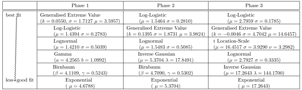
whole blood data are used. In table 1 the ve best tting distributions are shown.

Table 1: Ordering of best tting probability distributions

Phase 1 Phase 2 Phase 3

best t Generalised Extreme Value (k= 0.0550,σ= 1.7127µ= 3.5957)

Log-Logistic

(µ= 1.5464σ= 0.2810)

Log-Logistic

(µ= 2.7959σ= 0.1785) Log-Logistic

(µ= 1.4394σ= 0.2783)

Generalised Extreme Value (k= 0.1395σ= 1.8731µ= 3.9824)

Generalised Extreme Value

(k=−0.0046σ= 4.7042µ= 14.6457)

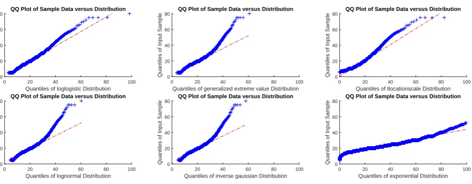
According to the results in table 1 the Generalised Extreme Value distribution and the Log-Logistic distribution

are the best t. To check how good those ts are, qq-plots of the phase 3 service times are shown in 2. The qq-plots

of phase 1/2 service times show similar results.

Quantiles of loglogistic Distribution

0 20 40 60 80 100

Quantiles of Input Sample 0 20 40 60

80 QQ Plot of Sample Data versus Distribution

Quantiles of generalized extreme value Distribution

0 20 40 60 80 100

Quantiles of Input Sample 0 20 40 60

80 QQ Plot of Sample Data versus Distribution

Quantiles of tlocationscale Distribution

0 20 40 60 80 100

Quantiles of Input Sample 0 20 40 60

80 QQ Plot of Sample Data versus Distribution

Quantiles of lognormal Distribution

0 20 40 60 80 100

Quantiles of Input Sample 0 20 40 60

80 QQ Plot of Sample Data versus Distribution

Quantiles of inverse gaussian Distribution

0 20 40 60 80 100

Quantiles of Input Sample 0 20 40 60

80 QQ Plot of Sample Data versus Distribution

Quantiles of exponential Distribution

0 20 40 60 80 100

Quantiles of Input Sample 0 20 40 60

80 QQ Plot of Sample Data versus Distribution

Figure 2: QQ-plots of tted data phase 3 service times

In gure 2 all qq-plots show a good t around the mean value of 17.2643 (standard deviation 6.1969). In section 5.1

and section 5.2 waiting time models are used with exponential service times. The qq-plot of the service time data

and the tted exponential distribution shows that an exponential service time can be assumed.

Also the p-values are calculated to check how good the distributions can be t to the data. To calculate p-values

the Chi-square goodness-of-t test is used. For all three phases and all distributions that are tted, the p-values

are smaller than the signicance level of 5%. This means that the null hypothesis, service time data comes

from distribution considered, is rejected. A possible reason for rejecting the null hypothesis is that the tted

distributions do not t the data good for high waiting time values.

5 Waiting time models

Since blood donors come voluntarily it is important to keep donors satised. For blood donors it is important that

the waiting time is low as possible. Therefore, to take this waiting time into account, two waiting time models are

treated in this section. These waiting time models give an indication for the possible waiting time. The models

are used later on to decide which time slots to open for whole blood donors to make an appointment and which to

close.

The donation process consists of three sequential phases. The donor has to complete phase one before phase two can

be started and phase two has to be completed before phase three can be started. This means the donation process

is a tandem queue consisting of three service points, with the exception that donors can leave the system before all

phases have been completed. At each service point there are one or more sta members to give service. A donor

can nish service without interruption, so the donation system is non-preemptive. One sta member is needed to

serve one donor. Currently, there are to types of donors, plasma and whole blood donors. Plasma donors have

absolute priority over whole blood donors, so a plasma donor has no waiting time, unless all sta members (of that

phase) are busy. The whole blood donors with appointment will have (absolute) priority over whole blood donors

without appointment. Therefore a plasma donor is in priority class one, a whole blood donor with appointment in

class two and a whole blood donor without appointment in class three.

5.1 Network of non-preemptive M/M/c queues with priorities

To be able to measure waiting time, the rst model to consider is the model of (27). In this article the

Laplace-Stieltjes transform of the waiting time

W

of a class-

k

customer in the non-preemptive priority

M/M/c

queue is

derived. All customers have the same mean service time. With this model the waiting time distribution of each

phase of the donation process can be determined. To use the model of (Yechiali1985) the assumption has to be made

that donors arrive according to a Poisson Process with rate

λ

, where

i

is the customer class. Another assumption

is that the service time of donors follows an exponential distribution, with rate

µ

. A donor is served by one of the

c

employees. The parameters in (3) are used for the model.

λ

=

X

i<k

λ

,

λ

=

n

X

i=1

λ

,

ρ

=

λ

(

cµ

)

,

ρ

=

λ

(

cµ

)

,

σ

=

X

i=1

ρ

,

ρ

=

λ

(

cµ

)

(3)

The Laplace-Stieltjes transform of the waiting distribution of a class-

k

donor derived in (27) is given by 4.

˜

W

(

s

) = (1

−

π

) +

π

·

(

cµ

(1

−

σ

)(1

−

γ

˜

(

s

))

s

−

λ

+

λ

˜

γ

(

s

)

)

(4)

π

=

(

λ/µ

)

c

c

!(1

−

ρ

)

X

i=0

(

λ/µ

)

i

!

+

(

λ/µ

)

c

!(1

−

ρ

)

(5)

˜

γ

(

s

) =

s

+

λ

+

cµ

−

[(

s

+

λ

+

cµ

)

2

₋

₄

_λ

a

cµ

]

2

λ

(6)

In (4)

π

is the probability that a donor has to wait.

The waiting time formula in 4 can be used for one phase of the donation process. For a donor it is important that

the total waiting time is low and not the waiting time of just one phase. If the density distribution of the waiting

time at each phase is known and the phases are considered independent, the density distribution of the total waiting

can be calculated by taking the convolution of the three density distributions. Alternatively, it is also possible to

multiply the Laplace-Stieltjes transform of the waiting time of the three phases. For the blood donation process

the assumption is made that the three phases are independent. The phases of the blood donation process are not

independent. The assumption of independent phases is discussed in (18). In section 7.1 a simulation model will

be dened to verify how good/bad this assumption is. The verication is done for a test case in section 8.2. The

Laplace-Stieltjes transform of the total waiting time distribution is then dened by (7).

˜

To measure the total waiting time for each donor class, the probability distribution of the total waiting time of

each donor class has to be calculated. This can be done by taking the inverse transform of the Laplace-Stieltjes

transform. The inverse transform can not be derived analytically. Therefore this has to be done numerically. For

the numeric inverse transform the Euler method of (31) is used. A disadvantage of calculating the inverse transform

numerically is the computation time. The numeric inverse transform process is so slow, that this method can not

be used for determining the a good appointment schedule. To many appointment schedule have to be evaluated.

If only one appointment schedule has to be evaluated, then this waiting time model can be used. To determine a

good appointment schedule a dierent waiting time model derived, this will be discussed in section 5.2.

5.2 Network of M/M/1 queues with capacity reservation

The waiting time model of section 5.1 can not be used for determining a good appointment schedule. Therefore a

second waiting time model is will be used for the determination of appointment schedules. The model to determine

a good appointment schedule will be discussed in section 6 and 6.3.

Similar to the model in section 5.1, donors arrive according to a Poisson process with rate

λ

for phase

p

and

donor class

k

. The donors of class

k

experience a service time which follows a exponential distribution with rate

¯

µ

at phase

p

. In phase one and two plasma donors and whole blood donors use the same resources and the need

same service, so the service rate is the same for both. In phase three plasma donors and whole blood donors are

separated, this means plasma donors do no have to be taken into account to calculate the waiting time for whole

blood donors in phase three of the donation process. So

µ

¯

is the service rate for whole blood donors. For each

phase each donor class is represented by a M/M/1 queue. In (8) the arrival rates of class

k

donors are dened for

each phase of the donation process. The probability that a donor does pass the medical check (phase 2) is

ρ

, so

ρλ

is the arrival rate for phase three.

λ

=

λ

,

λ

=

ρλ

(8)

Since at each phase of the donation process there are often more than one sta member the service rate has to be

adapted. Further the dierent priority classes have to be kept. Therefore the service rate of each donor class at each

phase of the donation process will be the total service capacity available. For each donor class the total available

capacity will be dierent, since the priority classes have to be taken into account. Since plasma donors have the

highest priority, they can use all capacity available, (9). The whole blood donors with appointment have less priority.

If all plasma donors are served then the remaining capacity is for the whole blood donors with appointment, (10).

The whole blood donors without appointment get the remaining capacity, not needed for plasma donors and whole

blood donors with appointment, (11).

¯

µ

=

C

µ

(9)

¯

µ

=

C

µ

−

λ

(10)

¯

µ

=

C

µ

−

λ

−

λ

(11)

For a M/M/1 queue the waiting time density function is known (12). The density function of (12) corresponds to

the waiting time probability distribution

P

(

W

> t

|

W

>

0) =

e

.

f

= ¯

µ

(1

−

ρ

)

e

−µ¯p,k(1−ρp,k)t

ρ

=

λ

¯

µ

(12)

Like in section 5.1 the assumption is made that the phases are independent. The phases of the blood donation

process are not independent. The assumption of independent phases is discussed in (18). In section 7.1 a simulation

model will be dened to verify how good/bad this assumption is. The verication is done for a test case in section

8.2. This means that the density function of the total waiting time can be calculated by taking the convolution

of

f

,

f

and

f

. The three density functions are simple enough to allow for analytical computation of

6 Schedule model

It has to be decided which time slots will be open for whole blood donors to make an appointment. For each week

the same slots will be open/closed for donors. For each slot it can be chosen if the slot is open or closed. Also

it can be choses how many appointment there can be made if a slot is open. The time slots open for making an

appointment for whole blood donation form a schedule. A schedule is one possibility of which slots are open/closed

and for how many appointments. Given that walk in donors show clear preferences for some times, we have to

carefully select the times at which an appointment can be made. To determine a good schedule, rst a schedule has

to be generated. This is explained in section 6.1. It is necessary to know how good certain schedules are. Therefore,

it has to be rated. In section 6.2 it is explained how schedules are given a rate.

6.1 Heuristic to generate schedules

To start the process of looking for good schedule, we will rst generate an initial schedule, and will then improve

this initial solution. To this end, the total total available capacity per time slot, per day is calculated. This is done

by calculating the maximum number of donors that can be serviced per phase (of the donation process) per time

slot, per day.

¯

C

=

C

·

µ

,

∀

i

= 1

, . . . ,

72

;

∀

d

= 1

, . . . ,

5

(13)

In (13)

C

is the total number of available sta members in phase

f

, at time slot

i

of day

d

. The service rate of

sta members of phase

f

is

µ

per 10 minutes. As there are 5 working days, maximal 72 time slots per day and

the donation process consists of 3 phases,

d

= 1

. . .

5

,

i

= 1

. . .

72

and

f

= 1

,

2

,

3

. If a location is not open at time

slot (i,d) than

C

= 0

,

∀

f

= 1

,

2

,

3

.

As mentioned in section 6.2, it has to be determined which time slots should be opened for whole blood donors to

make an appointments, and how many appointments should be allowed per time slot. To get the average arrival

rates, data of the arrivals in 2015 will be used. The average arrival rates will be computed for every donor type. In

the future Sanquin strives for a situation in which 80% of the whole blood donor should come with an appointment.

To reach this, we will start by summing up the arrival rates of the whole week. Then 80% of the total arrivals per

week is taken en round up to whole number. Equation (14) shows the arrival rates that will be used for the three

types of donors considered in this study.

λ

=

d

0

.

8

·

(

5

X

d=1 72

X

i=1

λ

)

e

;

λ

= 0

.

2

∗

λ

;

λ

(14)

In (14)

λ

is the averaged arrival rate of whole blood donors (100% walk in) per 10 minutes, as acquired from the

Data:λapp_{, λ}walkin i,d , λ

plasma

i,d ,C¯i,d, ρ(probability of passing medical check)

Result: Initial schedule S 1 s=0;

2 K is72x5matrix with all entries zero;

3 %while not all appointments planned 4 while s≤λappdo

5 % For all days 6 for d=1:5 do 7 % For all time slots 8 for i=1:72 do

9 % Remaining capacity phase 1

10 V1(i, d) = ¯C1,i,d−K(i, d)−λplasmai,d −λ walkin i,d ;

11 % Remaining capacity phase 2

12 V2(i, d) = ¯C2,i,d−K(i, d)−λplasmai,d −λ walkin i,d ;

13 % Remaining capacity phase 3, plasma donation separate from whole blood donation, so not considered 14 V3(i, d) = ¯C3,i,d−ρ·(K(i, d) +λwalkini,d );

15 % Determine which phase is the bottleneck 16 V(i, d) = min(V1(i, d), V2(i, d), V3(i, d))_;

17 end

18 end

19 % Choose the time slot with the most available capacity 20 (i∗, d∗) = maxi,dV;

21 % An appointment will be planned in the time slot with the most available capacity 22 K(i∗, d∗) =K(i∗, d∗) + 1;

23 % One appointment is planned 24 s=s+ 1;

25 end

26 % initial scheduleS=K_;

Algorithm 1: Generate initial schedule

To generate an initial schedule, algorithm 1 starts with an empty schedule K. Then for each time slot it calculates

the remaining capacity per phase if this schedule K is used, for phase one (V1), phase two (V2) and phase three

(V3). As the smallest remaining capacity, restricts the capacity of the system, the minimum of V1, V2 and V3

will be used to nd the best place to add an appointment. This minimum will be stored in V. Then the time slot

with the largest positive value for V will be selected, and an appointment will be added to this time slot. This

way, appointments are placed in time slots with a large excess capacity, which should result in a schedule with low

waiting times. Now one appointment is placed, the procedure in algorithm 1 repeats until all appointments are

placed in the schedule.

Data:S,C¯1,i,d, λapp, λwalkini,d , λ plasma

i,d , ρ, target

Result: Schedule K, u 1 % start with initial schedule 2 K=S;

3 % vectors which contain pair of indices. k1; 4 k2;

5 % For all days 6 for d=1:5 do 7 % For all time slots 8 for i=1:72 do

9 V1(i, d) = ¯C1,i,d−λplasmai,d −λ walkin

i,d ; % Determine the capacity available for whole blood donors with appointment for phase 1

10 V2(i, d) = ¯C2,i,d−λplasmai,d −λ walkin

i,d ; % Determine the capacity available for whole blood donors with appointment for phase 2

11 V3(i, d) = ¯

C3,i,d−ρ·λwalkin_i,d

ρ ; % Determine the capacity available for whole blood donors with appointment for phase 3

12 V(i, d) =bmin(V1(i, d), V2(i, d), V3(i, d))c;% Determine which phase is the bottleneck 13 end

14 end

15 % Determine how many appointments can maximally be scheduled, without having not enough service capacity 16 B=P

i,d1(V(i, d)≥0)·V(i, d);

17 % If more appointments can be scheduled than necessary 18 ifB > λapp_then

19 u= 1_;

20 Find the indicesi, d_{such that}V(i, d)≥1_{, put them in matrix C;}

21 M=max(V); % Maximal number of appointments that can be planned in one time slot 22 ifM >1_then

23 a= 2% If the maximal number of appointments that can be planned in one time slot is more than 1

24 end

25 ifM≤1then

26 a= 1% If the maximal number of appointments that can be planned in one time slot is less or equal as 1

27 end

28 % matrix with consists of indices of time slots where one extra appointment can be planned 29 Dene matrix D1, consisting of indices from C for whichS < a;

30 % matrix with consists of indices of time slots where one appointment will be removed 31 Dene matrix D2, consisting of indices from C for whichS≥a;

32 whilek1 ==k2do

33 %choose time slot where one appointment will be add 34 k1 is pair of indices randomly chosen from D1;

35 %choose time slot where one appointment will be removed 36 k2 is pair of indices randomly chosen from D2;

37 end

38 Remove one appointment from time slot indices from k2; 39 Add one appointment to time slot indices from k1; 40 end

41 % If as much appointments can be scheduled as necessary 42 ifB==λapp_then

43 Keep the initial schedule S; 44 u= 2_;

45 end

46 % If less appointments can be scheduled as necessary 47 ifB < λappthen

48 A=V; 49 % For all days 50 for d=1:5 do 51 % For all time slots 52 for i=1:72 do

53 V1(i, d) = ¯C1,i,d−λplasmai,d ;% Determine the capacity available for whole blood donors for phase 1

54 V2(i, d) = ¯C2,i,d−λplasmai,d ;% Determine the capacity available for whole blood donors for phase 2

55 V3(i, d) = C¯3,i,d_{ρ ;% Determine the capacity available for whole blood donors for phase 3}

56 V(i, d) =bmin(V1(i, d), V2(i, d), V3(i, d))c;% Determine which phase is the bottleneck

57 end

58 end

59 % Determine how much capacity there is for whole blood donors 60 B=P

i,d1(V(i, d)≥0)·V(i, d);

61 % If there is enough capacity for whole blood donors 62 ifB≥targetthen

63 u= 3;

64 K=B;

65 only whole blood donors with appointment; 66 end

67 % If there is not enough capacity for whole blood donors 68 ifB < targetthen

69 u= 4;

70 Find the indicesi, dsuch thatA(i, d)≥0, put them in matrix C;

71 ifλapp−B≥1then

72 M=max(V);

73 ifM >1then

74 a= 2

75 end

76 ifM≤1_then

Algorithm 2 starts in step 1 by choosing the initial schedule S as schedule. In line 4-12 the maximum number of

appointments that can be put in schedule K is calculated, given that the arrival rate has to be smaller than the

service capacity.

If there are more appointment possibilities than there are appointments needed, line 13-30, then it is best to look at

the time slots where there is enough capacity for all arriving plasma and whole blood donors without appointment

and at least one walk in donor with appointment. If there is enough capacity, waiting time will be lower than if an

appointment is planned in a time slot without enough capacity for all three donor types. Especially whole blood

donors without appointment will get a high waiting time if there is not enough capacity for all arriving donors. In

this case, an appointment will be moved from a time slot with a lot of appointments, line 28, to a time slot with

zero or one appointments, line 29.

If there are just as much appointment possibilities as there are appointments needed then the initial schedule S is

also the best schedule, step 31-33. In this case, appointments could only be moved to time slots where there is not

enough capacity for plasma donors, whole blood donors without capacity and one or more whole blood donors with

appointment. This will result in worse waiting time for whole blood donors with appointment, whole blood donors

without appointment or both donor types.

if there are less appointment possibilities than there are appointments needed, lines 34-67 will be used. In this

situation a combination of 80% whole blood donors with appointment and 20% whole blood donors without

ap-pointment is not possible, without creating some time slots that do not have enough capacity for all three donor

types. Therefore an alternative is checked with 100% whole blood donors with appointment. In lines 36-44 it is

calculated if this is possible. At least the target number of whole blood donations per week has to be reached, this

is checked in lines 45-48. In step 36-44 the maximum number of appointments is calculated that can be put in

schedule K if the arrival rate would be kept lower than the service capacity for each time slot consisting of plasma

and whole blood donors. If this target can not be reached, lines 49-67 compute the least bad schedule. Therefore

C is dened as in step 50. The same method is used in step 52-66 as in step 15-29.

6.2 Rating schedules

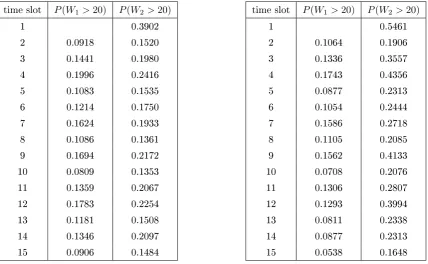
As explained in section 1.1, it has to be determined which time slots should be opened for appointments of whole

blood donors. For donors it is very important that the total waiting time is low. With the two waiting time models

from section 5, the probability of waiting longer than t minutes can be determined for each donor type

k

per time

slot. Each working day is divided in slots of 10 minutes and a location might be open between 8.00 and 20.00. For

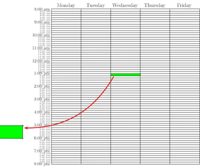
each of the slots for each of the days of the week, the waiting time probabilities are determined. This results in a

72

x

5

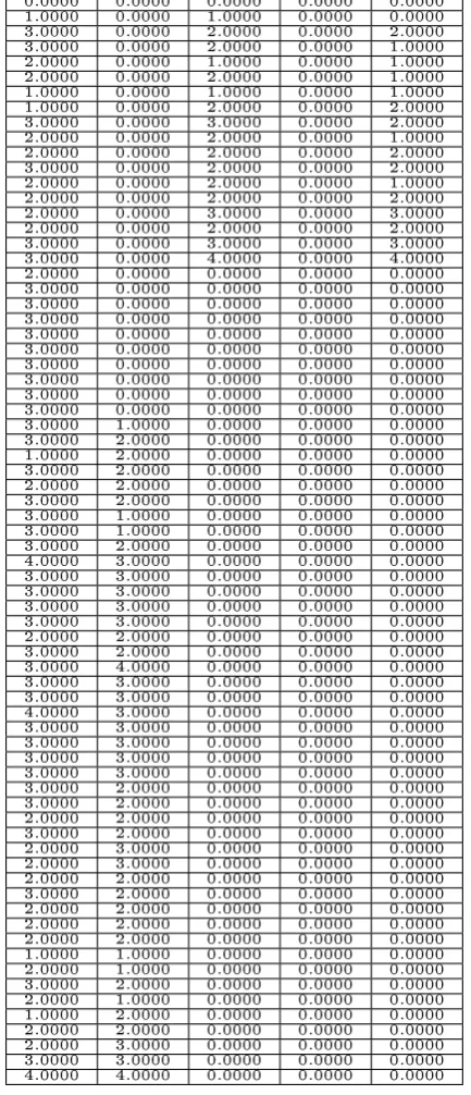
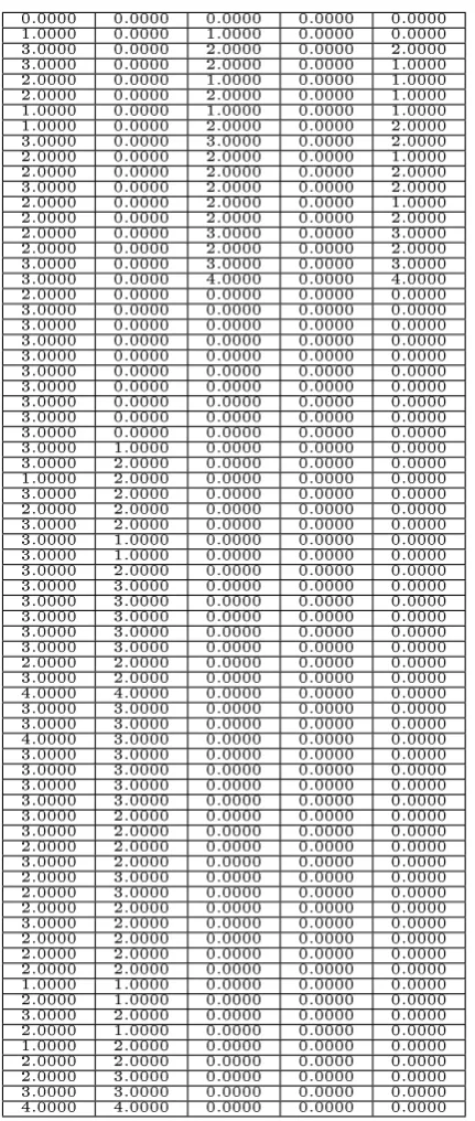
matrix

R

(for donor type

k

), with the columns representing the ve workings days (Monday-Friday) and the

Figure 3: Matrix to save the results one of the waiting time models

In gure 3 the results of one of the waiting time models of section 5 are saved in a matrix. As in gure 3, zoom in

to a time slot. In this case, we will use Wednesday from 13.00 till 13.10 as an example. If the location is not open

at that time slot no waiting probability has to be calculated. If the location is opened, the waiting model in section

5.1 has the restriction that the total arrival rate of all three donor types must be smaller than the service rate at

each phase of the donation process. The queuing model in section 5.2 has the restriction that the arrival rate of a

type

k

donor must be smaller than the service rate of a type

k

donor at each phase of the donation process. Both

restrictions are used to make sure there is enough capacity to service all the arriving donors. If these restrictions

are met then

R

(31

,

3)

has the value

P

(

W

> t

)

or

P

(

W

> t

|

W

>

0)

, respectively for the models of section 5.1

and 5.2. If the restrictions are not met then

R

(31

,

3)

is given the value 1.

To decide which schedule is best, it is necessary to grade a schedule. This is done with an cost function. For whole

blood donation with appointment the cost function 15 is used, for whole donation without appointment the cost

function 16.

5

X

d=1 72

X

i=1

1

(

center is open at time slot

(

i, d

))

·

[

R

(

i, d

)

|

{z

}

a

+

P enalty

(

R

(

i, d

))]

(15)

5

X

72

X

equation (15) and (16). If there is not enough capacity to service the arriving donors,

R

(

i, d

) = 1

(

k

= 2

,

3

). A

schedule with one time slot

R

(

i, d

) = 1

and one time slot

R

(

i, d

)

low is worse than a schedule with two time slots

R

(

i, d

)

average. To keep donors satised it is better that donors experience the same waiting time. As part a of

equation (15)/(16) is unable to distinguish between these to variants, a penalty is introduced. This corresponds to

the remaining part of the equation. Therefore a penalty is needed, other part of 15/16. Since whole blood donors

with appointment have priority over whole blood donors without appointment, the penalty for not having enough

capacity is higher for whole blood donors with appointment than for whole blood donors without appointment.

The appointments of plasma donors are made independently of the arrivals/appointments of whole blood donors.

This means that only the schedule for whole blood appointments can be used to reduce waiting time. Only the

time slots with low expected arrivals of plasma donors and walk in whole blood donors, will be opened for whole

blood appointments. This reduces the waiting time for both whole blood donors and plasma donors. A minimum

number of slots have to be opened and lled with appointments, otherwise the target, total number of donations

per week, is not reached. Plasma donors have higher priority than whole blood donors. The planning of plasma

donors can not be inuenced, it is a given. An cost function for plasma donors is therefore not necessary.

6.3 Heuristic to determine schedule

In section 6 it is explained how (week) schedules of appointments for whole blood donation are generated and

rated. Several schedules have to be generated, such that the best schedule can be chosen. To choose the best

schedule a rating is necessary. In this section a heuristic is given to determine a good enough schedule. Alternately

schedules are generated and rated, and checked if the newly generated schedule is better as the best schedule so

far.

The procedure in algorithm 3 is used to nd the best possible schedule.

Data:Cf,i,d, µf, λi,d, λplasmai,d , ρ, target, I

Result: Schedule SS

1 Determine initial schedule S with algorithm 1; 2 SS=S;

3 Calculate W1, this is the waiting probability matrixR1if the matrix SS is used;

4 Calculate W2, this is the waiting probability matrixR2if the matrix SS is used;

5 Rate schedule SS with equations 15 and 16; 6 for i=1:I do

7 Generate a schedule K and value of u with algorithm 2; 8 ifu== 2oru== 3then

9 stop for loop, best schedule has been found 10 end

11 ifu6= 2andu6= 3then

12 Calculate W1new, this is the waiting probability matrixR1if the matrix K is used;

13 Calculate W2new, this is the waiting probability matrixR2if the matrix K is used;

14 Rate schedule K with equations 15 and 16;

15 if Rates of schedule K lower than rates of schedule SS then

16 SS=K;

17 W1=W1new;

18 W2=W2new;

19 end

20 end 21 end

Algorithm 3: Procedure to nd good enough schedule

First an initial schedule S is calculated for the whole blood appointments, line 1 in algorithm 3. This initial schedule

is determined with algorithm 1. For schedule S the waiting time probability matrices,

R

and

R

are calculated, line

3-4. Section 6.2 describes how these matrices are determined. Depending on the available capacity in a time slot

an entry of the matrices

R

and

R

has the value one or, depending on the model,

P

(

W

> t

)

/

P

(

W

> t

|

W

>

0)

.

The matrices

R

and

R

are then rated with equations 15 and 16, in line 5.

I

determines the number of times the

heuristic will be applied. For a higher

I

, a better schedule will be found, but computational time will also increase.

are lower than those of schedule SS, then schedule K is accepted. If this is the case schedule K and the matrices

R

and

R

belonging to schedule K are saved, step 16-18. So the procedure in algorithm 3 is a repetition of generating

7 Simulation models

In this section two simulation models are introduced. The rst model is used to see how good/bad the assumption is

(see section 5) that the waiting time at the phases of the donation process are independent. The second simulation

model will give an indication of how the calculated appointment schedules (see section 6.3) will work out in practice.

Both models are made with Simulink (MATLAB R2016b).

7.1 First simulation model

With the waiting time models in section 5, the probability of waiting longer than t minutes can be computed for

each donor class and time slot. For each time slot, the waiting time probabilities are determined independent of

the other time slots of that day, and therefore do not take arrivals in other time slots into account. This property is

also put into the simulation model. For each time slot the corresponding waiting time probabilities are calculated

with the simulation model.

From section 6 the arrival rates, service rates and the number of sta members per phase are known. With the

heuristic in section 6.3 an appointment schedule can be computed. So the arrival rate of whole blood walk-in

donors for slot

i

on day

d

is

λ

i,d

and the arrival rate of plasma donors for slot

i

on day

d

is

λ

plasma

i,d

. The

elements of the schedule

SS

give the number of scheduled whole blood donors that will arrive at the beginning

of time slot

i

of day

d

. The service rate of one sta member at phase

f

is dened by

µ

and the number of sta

members working at phase

f

at time slot

i

of day

d

is given by

C

.

Just as for the waiting time models in section 5 the simulation model consist of the three donation phases. For each

phase the service time follows an exponential distribution with rate

µ

. Also the number of sta members,

C

,

is the same. The plasma and whole blood walk-in donors each arrive according to a Poisson Process with the rates

λ

and

λ

respectively.

For the simulation each day is divided in 72 time slots, the same number used in section 6. These time slots get

the index

i

_{. To calculate the waiting time probabilities of one time slot (section 5), a whole day at a donation}

location is simulated with the rates of (17).

¯

λ

=

λ

,

∀

i

= 1

, . . . ,

72

¯

λ

=

λ

,

∀

i

∗

_{= 1}

_{, . . . ,}

₇₂

¯

S

=

SS

,

∀

i

= 1

, . . . ,

72

¯

C

=

C

,

∀

i

= 1

, . . . ,

72;

∀

f

= 1

,

2

,

3

(17)

If the waiting time probabilities belonging to time slot

i

on day

d

have to be simulated than

¯

λ

i∗

is the arrival

rate (of Poisson process) of whole blood walk-in donors for time slot

i

of the simulation model. Further

λ

¯

is

the arrival rate (of Poisson process) of plasma donors for time slot

i

of the simulation model and

S

¯

is the number

whole blood donors with appointment, coming at the begin of time slot

i

of the simulation model. These arrival

rates are valid if the location considered is open at time slot

i

, if closed there are no arrivals. This simulation

model is in correspondence with the way waiting time probabilities are calculated for time slot

i

on day

d

with the

waiting time models in section 5. The dierence is that the phases of the blood donation process are dependent

for the simulation model. Also in the simulation model the priorities of donors are as in practice.To calculate

the waiting time probabilities belonging to time slot

i

of day

d

the simulation has to be run multiple times. The

method of Monte Carlo simulation is applied.

Data:C¯f,i∗, µf,λ¯walkini∗ ,λ¯plasma_i∗ ,S¯i∗, I

Result: chance1, chance2 1 K1=zeros(1,2);

2 K2=zeros(1,2); 3 for i=1:I do

4 Run simulation model with arrival ratesλ¯walkin_i∗ ,¯λplasma_i∗ ,S¯i∗, service ratesµfand number of sta membersC¯f,i∗;

5 Determine T1, that are the arrival times of all whole blood donors with appointment that have passed all phases; 6 Determine wait1, that are the waiting times of all whole blood donors with appointment that have passed all phases; 7 Determine T2, that are the arrival times of all whole blood donors without appointment that have passed all phases; 8 Determine wait2, that are the waiting times of all whole blood donors without appointment that have passed all phases;

9 Determine index1a, this is the number of whole blood donors with appointment that have passed all phases and had to wait longer than t minutes in this run of the simulation model;

10 Determine index1b, this is the number of whole blood donors with appointment that have passed all phases in this run of the simulation model; 11 chances1 =index1a/index1b_;

12 Determine index2a, this is the number of times that whole blood donors without appointment have to wait longer than t minutes in this run of the simulation model;

13 Determine index2b, this is the number of whole blood donors without appointment that have passed all phases in this run of the simulation model;

14 chances2 =index2a/index2b_; 15 if index1b>0 then

16 K1=K1+[index1a*chances1,index1a]; 17 end

18 if index2b>0 then

19 K2=K2+[index2a*chances2,index2a]; 20 end

21 end

22 chance1=K1(1,1)/K1(1,2); 23 chance2=K2(1,1)/K2(1,2);

Algorithm 4: Procedure to nd waiting time probabilities via simulation

Before running algorithm 4, it has to be decided for which time slot of a certain day the waiting time probabilities

have to be calculated via simulation. Then the input (17) is xed. As Monte Carlo simulation is applied, the

simulation is done

I

times, line 3-21 of algorithm 4. How to determine the value of I is explained in section 7.3.

If a simulation is done (line 4) then the arrival times and waiting times are known. The arrival times are assigned

to T1 and T2, line 5/7. The waiting times are assigned to wait1 and wait2, line 6/8. Only donors arriving during

opening hours are taken into account. In step 11 and step 14 the probability of passing all phases and waiting

longer than t minutes is determined. This probability is only valid for the arrival pattern of the just done run of

the simulation model. If the simulation model is run again dierent probabilities are used, the random number

generators get a new seed. Since the number of donors passing all phases is dierent each time the simulation model

is run, also

index

1

a/index

2

a

changes. The number of whole blood donors with/without appointment that have

passed all phases of the donation process and have to wait longer than t minutes is assigned to

index

1

a

,

index

2

a

respectively. The value

index

1

a/index

2

a

gives an indication of the statistical quality of the calculated probability

chances

1

/changes

2

. Therefore the probability

chances

1

/changes

2

has to be weighted with

index

1

a/index

2

a

,

index

1

a

∗

chances

1

/

index

2

a

∗

chances

2

is calculated. All weighted probabilities and weights are summed, step 16

and 19. The weighted average is the probability that was the aim of the algorithm, step 22-23.

7.2 Second simulation model

unpunctuality of plasma donors. If a simulation is run for day

d

, then the rst inter-arrival time of a plasma/whole

blood walk-in donor is according to the exponential distribution with arrival rate

λ

/

λ

. If donor number

n

of class

k

arrives than the inter-arrival time of donor number

n

+ 1

of class

k

is determined. Depending the time

slot in which donor

n

arrives, say it is time slot

i

, than the inter-arrival time of donor

n

+ 1

is calculated with

arrival rate belonging to time slot

i

of day

d

. The inter-arrival times of whole blood donors with appointment is

xed by appointment schedule

SS

.

Also in this simulation model each donor entering the blood donation location of the simulation will be assigned

attributes. Those attributes are: class, value to indicate if donor will pass medical test (Bernoulli distribution),

arrival time, service time phase 1, service time for phase 1 to 6, total sojourn time and total waiting time. The

output of the simulation model are the attribute values of all (whole blood) donors that have gone through all

phases of the donation process. The attribute values are in order of the arrival times of the donors. To calculate the

waiting time probabilities belonging to donors arriving in time slot

i

of day

d

Monte Carlo simulation is applied.

This procedure is given in algorithm 5.

Data:Cf,i,d, µf, σf, λwalkini,d , λ plasma i,d , SSi,d, I

Result: chance1, chance2 1 K1=zeros(72,2);

2 K2=zeros(72,2); 3 for i=1:I do

4 Run simulation model with arrival ratesλwalkin_i,d , λplasma_i,d , SSi,d, service time paratetersµf,σfand number of sta membersCf,i,d;

5 Determine T1, vector with the arrival times of all whole blood donors with appointment that have passed all phases; 6 Determine wait1, vector with the waiting times of all whole blood donors with appointment that have passed all phases; 7 Determine T2, vector with the arrival times of all whole blood donors without appointment that have passed all phases; 8 Determine wait2, vector with the waiting times of all whole blood donors without appointment that have passed all phases; 9 chances1=zeros(72,2);

10 chances2=zeros(72,2); 11 for j=1:size(T1) do

12 chances1(bT1(i)/10c+ 1,2) =chances1(bT1(i)/10c+ 1,2) + 1_;

13 if wait1(1,1,i)>t then

14 chances1(bT1(i)/10c+ 1,1) =chances1(bT1(i)/10c+ 1,1) + 1;

15 end

16 end

17 end

18 for j=1:size(T2) do

19 chances2(bT2(i)/10c+ 1,2) =chances2(bT2(i)/10c+ 1,2) + 1;

20 if wait2(1,1,i)>t then

21 chances2(bT2(i)/10c+ 1,1) =chances2(bT2(i)/10c+ 1,1) + 1;

22 end

23 end

24 end

25 for j=1:72 do

26 if chances(j,2)>0 then

27 K1(j,:)=K1(j,:)+[chances1(j,1)*(chances1(j,1)/chances1(j,2)),chances1(j,1)];

28 end

29 if chances(j,2)>0 then

30 K2(j,:)=K2(j,:)+[chances2(j,1)*(chances2(j,1)/chances2(j,2)),chances2(j,1)];

31 end

32 end 33 end

34 chance1=K1(:,1)./K1(:,2); 35 chance2=K2(:,1)./K2(:,2);

Algorithm 5: Procedure to get indication of waiting time probabilities in practice

For the Monte Carlo simulation, the simulation model will run

I

times, line 3-33. How to determine the value

of

I

is explained in section 7.3. First the simulation model will be run, line 4. The output of the simulation

model will be the arrival times and waiting of the donors that have passed all phases of the donation process. The

arrival times of the whole blood with/without appointment will be assigned to T1/T2 and the waiting times to

wait1/wait2, line 5-8. For each arriving whole blood donor with appointment, the donor is numbered with

i

, it

is determined in which time slot the arrival was, slot number

b

T

1(

i

)

/

10

c

+ 1

. For each time slot it is calculated