Original citation:
Stinner, Björn and Garcke, Harald. (2006) Second order phase field asymptotics for multi-component systems. Interfaces and Free Boundaries, Volume 8 (Number 2). pp. 131-157. ISSN 1463-9963
Permanent WRAP url:
http://wrap.warwick.ac.uk/63303
Copyright and reuse:
The Warwick Research Archive Portal (WRAP) makes this work by researchers of the University of Warwick available open access under the following conditions. Copyright © and all moral rights to the version of the paper presented here belong to the individual author(s) and/or other copyright owners. To the extent reasonable and practicable the material made available in WRAP has been checked for eligibility before being made available.
Copies of full items can be used for personal research or study, educational, or not-for profit purposes without prior permission or charge. Provided that the authors, title and full bibliographic details are credited, a hyperlink and/or URL is given for the original metadata page and the content is not changed in any way.
Publisher’s statement:
© 2007 EMS Publishing House.
A note on versions:
The version presented here may differ from the published version or, version of record, if you wish to cite this item you are advised to consult the publisher’s version. Please see the ‘permanent WRAP url’ above for details on accessing the published version and note that access may require a subscription.
SECOND ORDER PHASE FIELD ASYMPTOTICS FOR MULTI-COMPONENT SYSTEMS
HARALD GARCKE AND BJ ¨ORN STINNER
Abstract. We derive a phase field model which approximates a sharp interface model for solidification of a multicomponent alloy to second order in the interfacial thickness
ε. Since in numerical computations for phase field models the spatial grid size has to
be smaller than ε the new approach allows for considerably more accurate phase field
computations than have been possible so far.
In the classical approach of matched asymptotic expansions the equations to lowest order in ε lead to the sharp interface problem. Considering the equations to the next
order, a correction problem is derived. It turns out that, when taking a possibly non-constant correction term to a kinetic coefficient in the phase field model into account, the correction problem becomes trivial and the approximation of the sharp interface problem is of second order inε. By numerical experiments, the better approximation property is
well supported. The computational effort to obtain an error smaller than a given value is investigated revealing an enormous efficiency gain.
1. Introduction
In sharp interface approaches to solidification phase boundaries are modelled as hyper-surfaces across which certain quantities jump. In the last two decades also the phase field method has become a powerful tool for modelling the microstructural evolution during solidification (see [7, 25, 11, 8] for reviews). Instead of explicitly tracking the solid-liquid interface an order parameter is used. It takes different values in the phases and changes smoothly in the interfacial regions which leads to the notion of diffuse interface models. The typical thickness of the diffuse interface is related to a small parameter ε. In the limit asε→0 sharp interface models are recovered.
The relation between the phase field model and the free boundary problem is established using the method of matched asymptotic expansions. It is assumed that the solution to the phase field model can be expanded in ε-series in the bulk regions occupied by the phases (outer expansion) and, using rescaled coordinates, in the interfacial regions (inner expansion). To leading order in ε, a sharp interface problem is obtained. If we consider the phase field system as an approximation of the sharp interface problem it would of course be desirable that phase field solutions converge fast with respect to ε
to solutions to the sharp interface problem. This becomes even more important as in numerical computations the spatial grid size has to be chosen smaller than ε (see e.g. [14]). In this paper we are interested in phase field approximations of the sharp interface problem which are of second order, i.e., we aim for constructing phase field systems such
Date: September 7, 2005.
1991Mathematics Subject Classification. 82C26, 82C24, 35K55, 34E05, 35B25, 35B40, 65M06.
that the first order correction in theε-expansion vanishes. This would then lead to much more efficient numerical approaches for solidification.
The method is formal in the sense that, a posteriori, it is not controlled whether the asymptotic expansions really exist and converge. In the context of solidification it has been applied on models for pure substances [10, 26], alloys [30, 5], multi-phase systems [16], and systems with both multiple phases and components [17] in order to derive sharp interface limits (first order asymptotics). We remark that, in some cases, this ansatz has been verified by rigorously showing that, in the limit as ε →0, the sharp interface model is obtained from the diffuse interface model (see e.g. [1, 10, 12, 28]).
Our interest in the higher order approximation is motivated by the results obtained by Karma and Rappel [20] in the context of thin interface asymptotics where the interface thickness is small but remains finite. Their analysis led to a positive correction term in the kinetic coefficient of the phase field equation balancing undesirable O(ε)-terms in the Gibbs-Thomson condition and raising the stability bound of explicit numerical methods. Besides, the better approximation allows for larger values of ε and, therefore, for coarser grids. In particular, it is possible to consider the limit of vanishing kinetic undercooling. Almgren [2] extended the analysis to the case of different diffusivities in the phases and discussed both classical asymptotics and thin interface asymptotics. By choosing different interpolation functions for free energy density and internal energy density an approximation to second order can still be achieved but the gradient structure of the model and thermo-dynamical consistency are lost. Andersson [4] showed, based on the work of Almgren, that even an approximation of third order is possible by using high order polynomials for the interpolation. McFadden, Wheeler, and Anderson [24] used an approach based on an en-ergy and an entropy functional providing more degrees of freedom to tackle the difficulties with unequal diffusivities in the phases while avoiding the loss of the thermodynamical consistency. Again, both classical and thin asymptotics are discussed as well as the limit of vanishing kinetic undercooling. In a more recent analysis Ramirez et al. [27] considered a binary alloy also involving different diffusivities in the phases and obtained a better ap-proximation by adding a small additional term to the mass flux (antitrapping mass current, the ideas stem from [19]).
We aim to extend the results to general non-isothermal multi-component alloy systems allowing for arbitrary phase diagrams with two phases. The models studied in the literature usually use the free energy or the entropy as thermodynamical potentials (see e.g. [3, 26, 29, 30] and the discussion in [21]). It turns out that, in our context, the reduced grand canonical potential ψ (see [23]) is more appropriate for the analysis. To motivate this let us review some thermodynamics.
We will, for simplicity, consider a system with uniform density, which is in mechanical equilibrium throughout the evolution. Changes is pressure or volume are neglected. In this case, the Helmholtz free energy density f is an appropriate thermodynamical quantity to work with. It is conveniently written as a function of the absolute temperature T and the concentrationsc= (c(1), . . . , c(N))∈RN, its derivatives being the negative entropy density −s and the chemical potentials µ= (µ(1), . . . , µ(N))∈RN,
df =−s dT +µ·dc.
Here, the central dot denotes the scalar product on RN. The internal energy density is
grand canonical potential, we then obtain
dψ =d³f−µ·c
−T ´
=e d³−1 T
´
+c·d³µ T
´ ,
in particularu= (u(0),u˜) = (−T1,µ
T)∈R N+1
are the to (e,c)∈RN+1 conjugated variables. Assuming local thermodynamical equilibrium the vector u is continuous across the free boundary in a sharp interface model. This will be important in the matched asymptotic expansions studied later and therefore we will state the problem from the beginning in these variables. We refer to Appendix A for more details on the thermodynamical background.
Next, we will briefly state a sharp interface problem for a liquid-solid phase change in a non-isothermal multi-component system (cp. [17] for more details). Let Dl and Ds be the domains occupied respectively by the liquid phase and the solid phase and let Γ be the interface separating the phases. In Dl and Ds, conservation of mass and energy is expressed by the balance equations
∂tψ,u(i)(u) =−∇ ·Ji =−∇ ·
N
X
j=0
Lij∇(−u(j)), 0≤i≤N, (1)
where ψ,u(0) = e and ψ,u(i) = c(i) denote derivatives of ψ, the Ji are the fluxes, and L =
(Lij)i,j is a matrix of Onsager coefficients which may depend onu. Constitutive relations between ψ,L, and u may depend on the two phases s and l. On Γ it holds
u(i) is continuous, 0≤i≤N, (2)
[−Ji]ls·ν =
h
− N
X
j=0
Lij∇u(j)
il
s·ν =v[ψ,u(
i)(u)]l
s, 0≤i≤N, (3)
αv =σκ−[ψ(u)]ls, (4)
whereν is the unit normal on Γ pointing intoDl,vis the normal velocity into the direction
ν, σ is the surface tension, κ the curvature, α a kinetic coefficient, and [·]l
s denotes the jump of the quantity in the brackets, for example [ψ(u)]l
s =ψl(u)−ψs(u). Equations (2) and (3) are also due to conservation of mass and energy. The Gibbs-Thomson conditions (4) couples the motion of the phase boundaries to the thermodynamical quantities of the adjacent phases such that, locally, entropy production is non-negative. For the case of a system involving multiple phases this is shown in [17].
The above stated sharp interface model will be approximated by a phase field model of the form
ω∂tϕ =σ∆ϕ−σε12w0(ϕ) + 21εh0(ϕ)
¡
ψl(u)−ψs(u)
¢
, (5)
∂tψ,u(i)(u, ϕ) =∇ ·
N
X
j=0
Lij∇u(j), 0≤i≤N. (6)
The approximation of the sharp interface model has to be understood in the following sense: Assume that solutions (u, ϕ) to (5) and (6) can be expanded in ε-series of the form
u=u0+εu1+. . . , ϕ=ϕ0+εϕ1 +. . .
and similarly in the interfacial regions using coordinates which are partially rescaled in ε
(the expansions are precisely stated in Section 2 as well as the following matching pro-cedure). After matching the expansions, u0 and ϕ0 solve (1)-(4) where Dl = {ϕ0 = 1},
Ds={ϕ
0 = 0}, Γ is the set where ϕ0 jumps, and α is related to ω.
As long as the first order correction terms (u1, ϕ1) do not vanish the approximation of
the sharp interface model by the phase field model is said to be of order one. Otherwise it is (at least) of order two. To see whether this is the case one has to derive and analyze the equations fulfilled by (u1, ϕ1). Our result now reads as follows:
Main result: Consider a two-phase multi-component system with arbitrary phase diagram. Then there is a possibly non-constant correction term to the kinetic coefficientωsuch that the sharp interface model(1)-(4)is approximated by the phase field model (5), (6) to second order. The kinetic coefficient has the structure ω =ω0+εω1(u)where
ω1(u) = [ψ,u(u)]
l
s·L−1[ψ,u(u)]
l sC
with some constant C depending on the interpolation function h.
A new feature compared to the existing results in [2, 4, 20] is that, in general, this correction term depends on u, i.e. on temperature and chemical potentials. Indeed, up to some numerical constants, the latent heat appears in the correction term obtained by Karma and Rappel [20]. Analogously, the equilibrium jump in the concentrations enters the correction term when an isothermal binary alloy is investigated. But from realistic phase diagrams it can be seen that this jump depends on the temperature leading to a temperature dependent correction term in the non-isothermal case.
Our model will be described in Section 2. In Section 3 we will apply matched asymptotic expansions to deduce a linear parabolicO(ε)-correction problem. Given appropriate initial and boundary conditions, zero is a solution to the correction problem. By numerical simulations of suitable test problems we investigate the gain in efficiency due to the better approximation. For this purpose, numerical approximations of solutions to the phase field model with and without correction term are compared in Section 4.
2. Phase field model for multi-component systems
LetD⊂Rd, d= 1,2,3, be a spatial domain with Lipschitz boundary which is occupied by an alloy and let I = [0, tmax] be a time interval. Further, let N ∈ N be the number of components in the system.
Convention: Throughout this article, partial derivatives are sometimes denoted by subscripts after a comma. For example,ψ,uϕ(u, ϕ) denotes the second-order mixed
deriva-tive ofψ(u, ϕ) with u and ϕ. Vectors of the size N+ 1 are printed in bold face except for the derivatives of ψ, ψs, and ψl with respect to u. Tensors of the size (N + 1)×(N + 1) are underlined.
2.1. Motivation. The Allen-Cahn equation
ω0∂tϕ = ∆ϕ− 1
ε2w
models the motion of an interface between two phases; here, ϕ is a phase field variable. It describes the presence of one of the phases. In the regions occupied by a pure phases
ϕ takes values close to 0 or 1. These values are the absolute minima of the double-well potential w. In transition regions connecting these regions occupied by the pure phases
ϕ varies smoothly between 0 and 1 due to the diffusion term ∆ϕ. The transition region will turn out to have a thickness of orderε. By adding further terms a dependence of the interface motion on thermodynamical quantities can be modeled.
The above differential equation is coupled to balance equations for energy and mass. The thermodynamical potentials are postulated to be the derivatives of the entropy den-sity (see [17]), and for the fluxes we postulate linear combinations of the corresponding thermodynamical forces, hence with Onsager coefficientsLij we obtain
∂te=−∇ ·
³
L00(T,c, ϕ)∇
1
T +
N
X
j=1
L0j(T,c, ϕ)∇−
µ(j)
T ´
,
∂tc(i) =−∇ ·
³
Li0(T,c, ϕ)∇
1
T +
N
X
j=1
Lij(T,c, ϕ)∇−
µ(j)
T ´
whereT is the temperature andc= (c(1), . . . , c(N)) a vector of concentrations,c(i)describing
the presence of component i. Given the free energy density f = f(T,c), the chemical potential corresponding to component i is the derivative of f with respect to c(i), i.e.
µ(i)=f
,c(i). The internal energy density ise=f+sT,s=−f,T being the entropy density.
2.2. Model and assumptions. It turns out to be more appropriate to write down the above conservation laws in terms of the variablesu = (−1
T ,
µ
T) and to use the reduced grand canonical potential as the thermodynamical potential (see Appendix A for the thermody-namical relations). We define the set
ΣN :=nc= (c(1), . . . , c(N))∈RN : N
X
i=1
c(i) = 1o,
and identify its tangential space in every pointc with
TΣN :=nu˜ = (u(1), . . . , u(N))∈RN : N
X
i=1
u(i)= 0o.
Moreover we define
Y :=R×TΣN.
The problem then consists of finding smooth functions
ϕ :I×D→R, u= (u(0), . . . , u(N)) :I×D→Y that solve the partial differential equations
(ω0+εω1(u))∂tϕ= ∆ϕ− 1
ε2w
0(ϕ) + 1
2εh
0(ϕ)Ψ(u), (7)
∂tψ,u(i)(u, ϕ) =∇ ·
N
X
j=0
The first equation is a forced Allen-Cahn equation for the phase field variable ϕ. The coupling to the thermodynamical quantities via the last term in that equation will be clarified below. We are interested in the limit ε → 0. The function ω1 : Y → R is some
correction term in order to obtain quadratic convergence and will be determined later. The derivatives of the reduced grand canonical potential are the conserved quantities energy
e = ψ,u(0) and concentrations c(i) = ψ,u(i), 1 ≤ i ≤ N (see the Appendix A for the exact
relation between (e,c) and the derivatives ofψ with respect tou). The equations in (7) are the balance equations for these conserved quantities. Concerning all the other functions and constants appearing in the above equations we make the following definitions and assumptions:
A. ω0 is a positive constant.
B. w : R → R+ is some nonnegative smooth double well potential which attains its global minima in 0 and 1, more precisely we have
w(ϕ)>0 if ϕ6∈ {0,1},
w(0) =w(1) = 0, w0(0) =w0(1) = 0, w00(0) =w00(1)>0.
Besides w is symmetric with respect to 1
2, i.e. w( 1
2 +ϕ) =w( 1 2 −ϕ).
C. h:R→R is a monotone symmetric interpolation function between 0 and 1, i.e.
h(0) = 0, h(1) = 1, h(12 +ϕ) = 1−h(12 −ϕ), h0(ϕ)≥0.
Furthermore we require that
h0(0) =h0(1) = 0.
D. ψ : Y ×R → R is smooth and given as interpolation between the reduced grand canonical potentials of the two possible phases s and l, i.e.
ψ(u, ϕ) =ψs(u) + ˜h(ϕ)
¡
ψl(u)−ψs(u)
¢
with a function ˜h satisfying Assumption C. Observe that in the case ˜h 6= h the model lacks thermodynamical consistency, i.e. an entropy inequality might not hold (see [26, 20, 2]). In (7) we used the abbreviation
Ψ(u) := ψl(u)−ψs(u).
The function ψ is convex inu so that (8) becomes parabolic. We will frequently use
ψ(u, ϕ),ψs(u) and ψl(u) as a function for arbitraryu ∈RN+1 which motivates one to write down the partial derivative ψ,u(k)(u, ϕ). But all the results do not depend
on the extension as only arguments u∈Y and derivatives alongY will be used. E. The matrix L = (Lij)Ni,j=0 of Onsager coefficients is constant, symmetric, positive
semi-definite, and the kernel is exactly Y⊥ = span{(0,1, . . . ,1) ∈ RN+1}. Observe that then
N
X
i=1
Lij = 0, 0≤j ≤N ⇒ ∂t
à N X
i=1
ψ,u(i)(u, ϕ)
!
= 0 ⇒ ∂t(ψ,u(u, ϕ))∈Y.
Besides for each v ∈ Y the linear system Lξ = v has exactly one solution ξ ∈ Y
which we will denote with ξ=L−1v.
already been considered in [2]. Therefore, the analysis is restricted to this simple case.
2.3. Evolving curves. To relate the diffuse interface model to a sharp interface model, the method of formally matched asymptotic expansions will be used. The procedure is outlined with great care in [15, 13]. Here, we will only sketch the main ideas for the two-dimensional case, i.e. d= 2.
For someε >0 we will denote a smooth solution to (7) and (8) with (u(t, x;ε), ϕ(t, x;ε)). The family of curves
Γ(t;ε) := nx∈D: ϕ(t, x;ε) = 12o, ε >0, t∈I, (9)
is supposed to be a set of smooth curves in D. In addition, we assume that they are uniformly bounded away from ∂D and depend smoothly on (ε, t) such that ifε →0 some limiting curve Γ(t; 0) is obtained. WithDl(t;ε) andDs(t;ε) we denote the regions occupied by the liquid phase (where ϕ(t, x;ε) > 12) and the solid phase (where ϕ(t, x;ε) < 12) respectively.
Let γ(t, s; 0) be a parametrization of Γ(t; 0) by arc-length s for every t∈I. The vector
ν(t, s; 0) denotes the unit normal on Γ(t; 0) pointing intoDl(t; 0) andτ(t, s; 0) :=∂
sγ(t, s; 0) denotes the unit tangential vector. The orientation is such that (ν, τ) is positively oriented. We assume that the curves Γ(t;ε) can be parametrized over Γ(t; 0) using some distance function d(t, s;ε) by
γ(t, s;ε) :=γ(t, s; 0) +d(t, s;ε)ν(t, s; 0). (10)
Close to ε = 0 we assume that there is the expansion d(t, s;ε) = d0(t, s) +ε1d1(t, s) +
ε2d
2(t, s) +O(ε3). As d(t, s; 0)≡0 we conclude d0(t, s)≡0.
Also the curvature κ(t, s;ε) and the normal velocity v(t, s;ε) of Γ(t;ε) are smooth and can be expanded (see Appendix C). We get
κ(t, s;ε) =κ(t, s; 0) +ε¡κ(t, s; 0)2d1(t, s) +∂ssd1(t, s) ¢
+O(ε2), v(t, s;ε) =∂tγ(t, s;ε)·ν(t, s;ε) =v(t, s; 0) +ε∂◦d1(t, s) +O(ε2);
here, ∂◦ =∂
t−vτ∂s denotes the (intrinsic) normal time derivative, vτ =∂tγ ·τ being the non-intrinsic tangential velocity (cp. Appendix B).
2.4. Definition of outer variables. We suppose that in each domain E such that its closure E with respect to the topology on Rd fulfills E ⊂ D\Γ(t; 0) the solution can be expanded in a series close to ε= 0 (outer expansion):
u(t, x;ε) = K
X
k=0
εkuk(t, x) +O(εK+1), ϕ(t, x;ε) = K
X
k=0
εkϕk(t, x) +O(εK+1). (11)
Near Γ(t; 0), we can define the coordinates (s, r), r being the signed distance of x from Γ(t; 0) (positive into direction ν, i.e. if x ∈ Dl(t; 0)). Hence, in a neighborhood of Γ(t; 0) we can write for r6= 0
ˆ
2.5. Definition of inner variables. Let z be the 1
ε-scaled signed distance of x from Γ(t; 0), i.e. z = rε, and let U(t, s, z;ε) := ˆu(t, s, r;ε), Φ(t, s, z;ε) := ˆϕ(t, s, r;ε). We now suppose that we can expand U and Φ in these new variables as follows:
U(t, s, z;ε) = K
X
k=0
εkUk(t, s, z) +O(εK+1), (13)
Φ(t, s, z;ε) = K
X
k=0
εkΦk(t, s, z) +O(εK+1). (14)
2.6. Matching conditions. For the two expansions for uto match in the limit as ε→0 there are certain conditions (see Appendix D for the derivation): As z → ±∞ for all
i∈ {0, . . . , N}
U(0i)(z)≈u(0i)(0±), (15)
U(1i)(z)≈u(1i)(0±) + (∇u(0i)(0±)·ν)z, (16)
∂zU(1i)(z)≈ ∇u (i)
0 (0±)·ν, (17)
∂zU(2i)(z)≈ ∇u (i)
1 (0±)·ν+ ¡
(ν· ∇)(ν· ∇)u0(i)(0±)¢z (18)
and analogously for Φ and ϕ. Here, for a function g(t, x) = ˆg(t, s, r),
g(0+) := lim
r&0ˆg(t, s, r), g(0
−) := lim
r%0gˆ(t, s, r),
wherer= dist(x,Γ(t; 0)). Remember that r >0 if and only ifx∈Dl(t; 0), and that r <0 if and only if x∈Ds(t; 0).
3. Asymptotic analysis
3.1. Outer solutions. In the region away from Γ(t; 0) we plug the expansions (11) into the differential equations (7) and (8). All terms that appear are expanded in ε.
To leading order O(ε−2) we obtain from (7) the identity 0 = −w0(ϕ
0). But the only
stable solutions to this equation are the minima of w, hence ϕ0 ≡0 or ϕ0 ≡1. We define
Ds(t; 0) as the set of all points with ϕ
0 = 0 and similarly Dl(t; 0) with ϕ0 = 1.
To the next order O(ε−1) we obtain
0 = −w00(ϕ0)ϕ1+
1 2h
0(ϕ
0)Ψ(u0). (19)
As ϕ0 = 0 or = 1, using the Assumptions B and C we obtain ϕ1 ≡ 0 as the only solution.
To leading order O(ε0) we obtain from (8), written as a vectorial equation,
∂t(ψ,u(u0, ϕ0)) = L∆u0. (20)
Depending on ϕ0 we have ψ,u(u0, ϕ0) = (ψl),u(u0) or ψ,u(u0, ϕ0) = (ψs),u(u0). In both
cases (20) is a parabolic equation foru0 by Assumption D.
To order O(ε1) we obtain
∂t
¡
(ψ,uu)(u0, ϕ0)u1
¢
=L∆u1 (21)
where we already made use of ϕ1 ≡0. Assumption D states that ψ is convex so that (21)
To determine boundary conditions for (20) and (21) on Γ(t; 0) we plug the expansions (13) and (14) into the differential equations.
3.2. Inner solutions to leading order. In Appendix B we describe how the derivatives with respect to (t, x) transform into derivatives with respect to (t, s, z). To leading order
O(ε−2) we get from (7)
0 =∂zzΦ0−w0(Φ0). (22)
By (9) and the assumption that (14) holds true forε= 0 we have Φ0(0) = 12. The matching
conditions (15) imply
Φ0(t, s, z)→ϕ(t, s; 0+) = 1 as z → ∞,
Φ0(t, s, z)→ϕ(t, s; 0−) = 0 as z → −∞.
Therefore Φ0(z) only depends onz. Furthermore Φ0 is monotone, approximates the values
at±∞ exponentially fast and fulfills Φ0(−z) = 1−Φ0(z).
For the conserved variables we get from (8)
0=L∂zzU0. (23)
Using Assumption E we have ∂zzU0 =L−10 =0 inY so that U0 is affine linear in z. By
the matching conditions (15), U0 has to be bounded as z → ±∞, hence we see that U0
must be constant in z which means U0 = U0(t, s). The matching condition (15) implies
that U0(t, s) is exactly the value of u0 in the point γ(t, s; 0)∈ Γ(t; 0) from both sides of
the interface. In particular,
u0 is continuous across the interface Γ(t; 0). (24)
3.3. Inner solutions to first order. To order O(ε−1) equation (7) yields
−ω0v∂zΦ0 =∂zzΦ1−κ∂zΦ0−w00(Φ0)Φ1+ 12h0(Φ0)Ψ(U0). (25)
From the solution to (19) we get ϕ1(t, s,0±) = 0. Besides ∇ϕ0(t, s,0±)· ν = 0 as ϕ0
is constant. Due to the matching conditions (16) we have Φ1 → 0 as z → ±∞. The
operator L(Φ0)b = ∂zzb−w00(Φ0)b is self-adjoint with respect to the L2-product over R.
Differentiating (22) with respect toz we obtain that∂zΦ0 lies in the kernel ofL(Φ0). Since
Φ0(−z) = 1−Φ0(z) we get with the help of Assumption C that ∂zΦ0 and h0(Φ0) are even,
hence (25) allows for an even solution and in the following we will assume that Φ1 is even.
We can deduce a solvability condition by multiplying the equation with ∂zΦ0 and
inte-grating over R with respect toz:
0 =
Z
R ¡
(κ−ω0v)(∂zΦ0(z))2− 12Ψ(U0)h0(Φ0(z))∂zΦ0(z) ¢
dz = (κ−ω0v)I−12Ψ(U0) (26)
where
I =
Z
R
(∂zΦ0)2dz.
The system (8) becomes to the order O(ε−1)
−v∂zψ,u(U0,Φ0) =−v∂z
¡
(ψs),u(U0) + ˜h(Φ0)Ψ,u(U0)
¢
As U0 =U0(t, s) we obtain Ψ,u(U0) = [ψ,u(u0)]
l
s = (ψl),u(u0)−(ψs),u(u0) for all z. We
integrate two times with respect to z and get
U1 =−L−1 ³
v Z z
0
ψ,u(U0,Φ0)dz0−Az
´
+ ¯u (27)
∼ −L−1³v(ψl),u(U0)z−Az−v[ψ,u(u0)]
l sH˜
´
+ ¯u as z → ∞
∼ −L−1³v(ψs),u(U0)z−Az−v[ψ,u(u0)]
l sH˜
´
+ ¯u as z → −∞
where A∈R×ΣN (observe that thenvψ,u−A∈Y which allowed us to use Assumption E to invert L) and ¯u∈Y are two integration constants and
˜
H =
Z ∞
0
(1−h˜(Φ0(z)))dz = Z 0
−∞
˜
h(Φ0(z))dz.
Here, we used the fact that Φ0converges to constants exponentially fast, so that the integral Rz
0 has been replaced by R∞
0 while the linear terms remain. Using (16) we derive
u1(t, s,0±) = ¯u+vL−1[ψ,u(u0)]
l
sH˜ (28)
which means, in particular, that
u1 is continuous across Γ(t; 0). (29)
With (17) the following jump condition is obtained at the interface:
[−L∇u0]ls·ν :=−L∇u0(t, s,0+)·ν+L∇u0(t, s,0−)·ν
=³v(ψl),u(u0)−A
´
−³v(ψs),u(u0)−A
´
=v[ψ,u(u0)]
l
s. (30)
3.4. Inner solutions to second order. Using the fact that Φ0 only depends on z the
phase field equation to order O(ε0) gives
−ω0v∂zΦ1−ω1(u0)v∂zΦ0−ω0(∂◦d1)∂zΦ0
=∂zzΦ2−w00(Φ0)Φ2+ (∂sd1)2∂zzΦ0−κ2(z+d1)∂zΦ0−∂ssd1∂zΦ0+
−κ∂zΦ1−12w000(Φ0)(Φ1)2+12Ψ(U0)h00(Φ0)Φ1+12Ψ,u(U0)·U1h0(Φ0).
To guarantee that Φ2 exists there is again a solvability condition which is obtained by
multiplying with ∂zΦ0 and integrating over R with respect to z. The Φ1-terms in this
condition vanish as can be seen as follows:
Z
R ³
(κ−ω0v)∂zΦ1+12w000(Φ0)(Φ1)2− 12Ψ(U0)h00(Φ0)Φ1 ´
∂zΦ0dz
=
Z
R ³
(κ−ω0v)∂zΦ1∂zΦ0−w00(Φ0)Φ1∂zΦ1+ 12Ψ(U0)h0(Φ0)∂zΦ1 ´
dz
=2(κ−ω0v) Z
R
∂zΦ1∂zΦ0dz− Z
R
where we used (25) to obtain the last identity. Since∂zΦ1·∂zΦ0 and ∂zzΦ1·∂zΦ1 are odd
the integrals in the last line vanish. Defining the constants
H :=
Z ∞
0
z∂z(h◦Φ0)(z)dz =− Z 0
−∞
z∂z(h◦Φ0)(z)dz,
J :=
Z ∞
0
∂z(h◦Φ0)(z) Z z
0
(1−(˜h◦Φ0)(z0))dz0dz
=
Z 0
−∞
∂z(h◦Φ0)(z) Z 0
z
(˜h◦Φ0)(z0)dz0dz
and using (27) for the remaining U1-term, a short calculation shows
−
Z
R 1
2Ψ,u(U0)·U1∂z(h◦Φ0)dz
=− 1
2[ψ,u(u0)]
l s·
³
¯
u−L−1[ψ,u(u0)]
l
sH+L−1[ψ,u(u0)]
l s2J
´
=− 1
2[ψ,u(u0)]
l
s·u1+v[ψ,u(u0)]
l
s·L−1[ψ,u(u0))]
l s
(H+ ˜H−2J) 2
where we used (28) to get the last equality. The whole solvability condition then becomes
0 =£−ω0∂◦+∂ss+κ2
¤
d1I− 12[ψ,u(u0)]
l su1
+v³−ω1(u0)I+ [ψ,u(u0)]
l
s·L−1[ψ,u(u0)]
l
sH+ ˜H2−2J ´
. (31)
We remark that∂◦d
1 and (∂ss+κ2)d1 are the first order corrections of the normal velocity
and the curvature of Γ(t, s;ε) (see Appendix C).
In the following, whenever we will evaluate ψ and its derivatives at (U0,Φ0) this will
be denoted by a superscript 0. The conservation laws (8) yield to orderO(ε0)
−v∂z(ψ,0uuU1+ψ
0
,uϕΦ1) +∂
◦ψ0 ,u−(∂
◦d
1)∂zψ,0u =L(∂zzU2−κ∂zU1+∂ssU0) (32)
where we used thatU0 does not depend onz. Integrating once with respect to z leads to
−L∂zU2 =v∂z
¡
ψ,0uuU1+ψ0,uϕΦ1
¢
−B
| {z }
(i)
+
Z z
0
((∂◦d1)∂zψ,0u−∂
◦ψ0 ,u)dz
0
| {z }
(ii)
−κLU1 | {z } (iii)
+L∂ssU0z (33)
where B ∈ Y is an integration constant. We want to derive a correction to the jump condition (30), i.e. a jump condition for u1. Therefore we are interested in the terms
contributing to ∇u1 ·ν in (18). Applying (16) to Φ1,U1 and using the fact that ˜h0(0) =
˜
h0(1) = 0 we see that
(i) ∼v(ψl),uu(u0)u1−B+ (. . .)z asz → ∞,
Furthermore
(ii) = (∂◦d1)(ψ,0u
¯ ¯z
0)− Z z
0
[∂◦((ψs)0,u) + (∂
◦Ψ0
,u)(˜h◦Φ0)(z
0)]dz0
∼ 1
2(∂◦d1)[ψ,u(u0)]
l
s−(∂◦(ψl),u(u0))z+∂◦[ψ,u(u0)]
l
sH˜ asz → ∞, ∼ −1
2(∂◦d1)[ψ,u(u0)]
l
s−(∂◦(ψs),u(u0))z+∂◦[ψ,u(u0)]
l
sH˜ asz → −∞ where for the first term the symmetry of ˜hin Assumption C has been used. In (iii) we use (28) again to obtain
(iii) =κLu1(t, s,0) + (. . .)z as z→ ±∞.
Finally, using (29), we get for the first order correction of the jump condition (30) at the interface:
[−L∇u1]ls·ν =v[ψ,uu(u0)]
l
s·u1+ (∂◦d1)[ψ,u(u0)]
l
s. (34)
3.5. Summary of the leading order problem and the correction problem. The problem to leading order consists of the bulk equation (20) which is coupled to the condi-tions (24), (30) and (26) on Γ(t; 0):
(LOP) Find a function u0 : I ×D → Y and a family of curves {Γ(t; 0)}t∈I separating D into two domains Dl(t; 0) and Ds(t; 0) such that
∂t((ψl),u(u0)) =L∆u0, inD
l(t; 0), t ∈I, ∂t((ψs),u(u0)) =L∆u0, inD
s(t; 0), t ∈I,
and such that on Γ(t; 0) there holds for all t∈I:
u0 is continuous,
[−L∇u0]ls·ν =v[ψ,u(u0)]
l s,
ω0v =κ−
1
2I[ψ(u0)]
l s
where ν is the unit normal to Γ(t; 0) pointing into Dl(t; 0). If we choose
ω1 =ω1(u0) := [ψ,u(u0)]
l
s·L−1[ψ,u(u0)]
l s
H+ ˜H−2J
2I (35)
then the correction problem consisting of (21), (29), (34) and (31) reads as follows: (CP) Let (u0,{Γ(t; 0)}t) be a solution to (LOP) and let l(t) be the length of Γ(t; 0) and setSI ={(t, s) :t∈I, s∈[0, l(t))}. Then we need to find functions
u1 :I×D→Y and d1 :SI →R such that
∂t((ψl),uu(u0)u1) =L∆u1, in D
l(t; 0), t ∈I, ∂t((ψs),uu(u0)u1) =L∆u1, in D
s(t; 0), t ∈I
and such that on Γ(t; 0) there holds for all t∈I:
u1 is continuous,
[−L∇u1]ls·ν =v[ψ,uu(u0)]
l
su1+ (∂◦d1)[ψ,u(u0)]
l s,
ω0(∂◦d1) = (∂ss+κ2)d1−
1
2I[ψ,u(u0)]
Obviously, (u1, d1) ≡0 is a solution given appropriate boundary conditions on ∂D. If
this solution is unique then the leading order problem is approximated to second order in
ε by the phase field model. The calculation in Appendix C shows that (CP) is in fact the linearization of (LOP). We point out that the choice (35) is crucial in order to guarantee that the undesired terms in (31) vanish.
Remark: If the diffusivity matrix L depends on u then equation (32) becomes
−v∂z(ψ,uu
0U
1+ψ0,uϕΦ1) +∂
◦ψ0 ,u−(∂
◦d
1)∂zψ,0u=L(U0)∂zzU2
+∂z
¡
L,u(U0)U1∂zU1
¢
+L,u(U0)(∂sU0)
2 +L(U
0)∂ssU0−κL(U0)∂zU1
resulting in
−L∂zU2 = (i) + (ii)−κL(U0)U1
| {z }
=(iii)
+L,u(U0)·U1∂zU1
| {z }
=:(iv)
+¡L,u(U0)(∂sU0)
2+L(U
0)∂ssU0 ¢
z
instead of (33). The matching conditions (15), (16) and (17) yield
(iv) =L,u(u0)·u1∇u0(0
±)·ν+ (. . .)z as z → ±∞.
This leads to an additional term in the jump condition of the correction problem. The condition (34) now reads
[−L(u0)∇u1−L,u(u0)·u1∇u0]
l
s·ν=v[ψ,uu(u0)]
l
su1+ (∂◦d1)[ψ,u(u0)]
l s,
but this is still consistent with the above statement that (CP) is the linearization of (LOP) as the additional term results from expanding L in a straightforward way.
4. Numerical simulations
Numerical simulations were performed in order to show that convergence to second or-der indicated by the analysis can really be obtained. For this purpose, we analyzed the
ε-dependence of numerical solutions to the phase field system and compared the numerical solutions with analytical solutions to the sharp interface problem if available. The differ-ential equations of the phase field system were discretized in space and time using finite differences on uniform grids with spatial mesh size ∆x and time step ∆t. The update in time was explicit, and to guarantee stability we chose ∆t . ∆x2. If not otherwise stated
we decreased the mesh size ∆x until we were sure that the error due to the discretization became inessential.
The order of convergence can be estimated by the following procedure: Assuming that the ε-dependence of the error can approximately be expressed by
Err(ε) =err εk+ higher order terms
with a constanterr and an exponentk > 0 which we are interested in. Given some m >1 (we often used m=√2) one can derive up to higher terms
Err(ε)−Err(mε)
Err(ε
m)−Err( ε m2)
= (m1)−k =mk (36)
4.1. Scalar case in 1D. Let d = 1 and N = 1, i.e. we consider a pure material. We set
u=u(0) and postulate the reduced grand canonical potential
ψ(u, ϕ) = 12cvu2+λ(um−u)(1−h(ϕ)), i.e. Ψ(u) =λ(u−um),
where λ, um and cv are constants. Choosing w(ϕ) = 92ϕ2(1−ϕ)2 as double well potential we obtain:
ε(ω0+εω1)∂tϕ=εσ∂xxϕ−9εσϕ(1−ϕ)(1−2ϕ) + 12λ(u−um)h0(ϕ), (37)
∂tψ,u=∂t(cvu−λ(1−˜h(ϕ))) = K∂xxu. (38)
This system differs from typical phase field systems (see e.g. [26]) by the term εω1. With
these equations the following sharp interface problem is approximated:
cv∂tu=K∂xxu, x6=p(t),
u is continuous,
λp0(t) = [−K∂xu]ls, x=p(t),
ω0p0(t) =λ(um−u), x=p(t),
wherep(t) denotes the position of the interface at timet. Imposing the boundary condition
u→u∞ asx→ ∞ there is the following travelling wave solution: Settingui =c−v1λ+u∞
we define
p(t) =v t=ω−01λ(um−ui)t, (39)
u=ui, x≤v t, (40)
u=u∞+ (ui−u∞) exp
¡
−K−1cvv(x−v t)
¢
, x > v t. (41)
Choosing ˜h(ϕ) =h(ϕ) =ϕ2(3−2ϕ) we compute I = 1
2,H+ ˜H−2J = 19
90. Furthermore if
λ = 0.5, um =−1.0, u∞ =−2.0, cv = 1.0, ω0 = 0.25, K = 1.0, σ= 1.0
we obtain the velocity v = 1.0, the value ui = −1.5 at the interface and by (35) the correction term ω1 ≈0.013194444.
We solved the differential equations on the time interval I = [0,0.1] for several values for ε. We chose Dirichlet boundary conditions for u given by the travelling wave solution (40),(41) to the sharp interface model and homogeneous Neumann boundary conditions for ϕ. To initialize ϕ we set
ϕ(0, x) := 1
2(1 + tanh( 3
2z)) = Φ0(z), z = x−x0
ε (42)
with some suitable initial transition point x0 such that the transition region (the set {ϕ ∈
(δ,1−δ)}for some smallδ, e.g. δ= 10−3) remains away from the outer boundary during the
evolution. The function Φ0 is the solution to (22) with the boundary conditions Φ0(z) →
0,1 asz → ∞,−∞. Initial values foruwere obtained by matching outer and inner solution to leading and first order obtained from the asymptotic expansions (see e.g. [22])
u(0, x) =u0(0, x) +εu1(0, x) +U0(0, z) +εU1(0, z)−common part.
The function u0(0, x) has the profile of the travelling wave solution:
u0(0, x) = (
u∞+ (ui−u∞) exp(−cKvv(x−x0)), x > x0,
ui, x≤x0.
As we want u1 ≡ 0 to be a solution to the correction problem we chose u1(0, x) = 0.
By equations (23) and (24), U0 ≡ ui is the interface value which is constant in normal direction. Equation (17) implies ∂zU1(z)→ ∇ ·u0(x−0) = 0 as z → −∞. As u1(0, x) = 0
we have ¯u=−KvλH˜ by (28). With (27) we see that A=v(ψs),u(U0) which yields
U1(0, z) = Kv (
λ−z+R0z(1−˜h◦ϕ0)(z0)dz0−H,˜ z >0,
λRz0(˜h◦ϕ0)(z0)dz0−H,˜ z <0.
The common part is ui− v λKz if z >0 and ui if z <0.
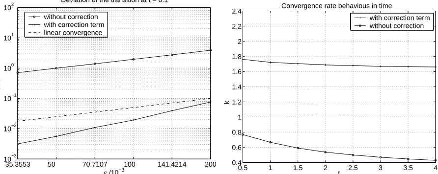
The phase boundaries {ϕ = 12} were determined by linearly interpolating the values at the grid points. Subtracting from the computed transition point the exact position given by (39) we got up to the sign the values in Figure 1 on the left. We found that when considering the correction term the interface was too slow but the numerical results indicated a quadratic convergence. Without the correction term ω1 the interface was too
fast and larger errors occurred indicating only linear convergence in ε. Similar results concerning the order of convergence hold true if
u(0, x) =u0(0, x) or ϕ=χ[x0,∞]
was chosen as initial data instead of the above smooth functions. The only difference is that then the errors are larger.
In the above simulations, the transition regions were resolved by more than 100 grid points to determine the error and the convergence behavior accurately. In applications, such resolutions of the interface are much too costly. Therefore, we simulated the same problem over the larger time intervalI = [0,8.0] with much less grid points in the interface. We found that theε/∆x ratio should be at least 5√2. The deviations at t= 8.0 are given in the following table:
ε 0.4 0.4/√2 0.2 0.2/√2 0.1 0.1/√2 0.05 with correction -0.0601 -0.0354 -0.0280
without corr. 0.5867 0.4155 0.2867 0.2020 0.1355 0.0948 0.0502 Again the errors are much larger without correction term. To get an error as obtained with correction term we need to take ε and ∆x eight times smaller. If explicit methods are used the expenditure becomes 8 times larger if the grid constant is halved due to the stability constraint ∆t.∆x2 for the time step. Hence, in our example, the costs without
the correction term are 83 = 512 times larger to obtain the same size of the error.
4.2. Scalar case in 2D. Now, letN = 1 and d= 2 and consider the same reduced grand canonical potential as in Subsection 4.1. Instead of the smooth double well potential we used the obstacle potential
wob(ϕ) =
( 8
π2ϕ(1−ϕ), 0≤ϕ ≤1,
∞, elsewhere.
35.3553 50 70.7107 100 141.4214 200 10−3
10−2 10−1 100 101 102
Deviation of the transition at t = 0.1
ε /10−3
error
without correction with correction term linear convergence
0.5 1 1.5 2 2.5 3 3.5 4
0.4 0.6 0.8 1 1.2 1.4 1.6 1.8 2 2.2 2.4
t
Convergence rate behavious in time
k
[image:17.595.81.527.103.281.2]with correction term without correction
Figure 1. On the left: deviations of the phase boundaries measured from the exact interface position given by (39) over ε; the resolution of the tran-sition region is very fine such that the error caused by the discretization is negligible; the dashed line corresponds to a linear convergence behavior inε. On the right: behavior of the numerically computed convergence rates (cp. (36)) in time for the angleβ = 15◦ (see Section 4.2).
We chose the following constants:
λ= 0.5, um = 2.0, cv = 1.0, ω0 = 0.25, K = 0.1, σ= 0.1.
We simulated the evolution of a radial interface. Initially, for ϕ we used the profile
ϕ(0, x) =
0, −∞< z ≤ −π82,
1
2(1 + sin( 4z
π)), − π2
8 ≤z≤ π2
8 ,
1, π82 ≤z <∞,
z = r−r0
ε ,
which is the solution to the variational inequality corresponding to (22) when restricted to a radial direction. Here, r = px2+y2 is the radius and we chose r
0 = 0.8. With
˜
h(ϕ) = h(ϕ) = ϕ2(3−2ϕ) we get the constants I = 1
2, H + ˜H −2J = 23π2
1024 and hence
ω1 = λ
2
K
H+ ˜H−2J
2I ≈ 0.554201419. For u initially the 1D profile (43) of the travelling wave solution in Subsection 4.1 in radial direction was used. As in the 1D case ui = −1.5,
v = ω0
λ(um−ui) = 0.25 and u∞=−2.0.
We considered the domain D = [0,8]2 and chose the grid constant ∆x = 0.02. At
different times we measured the distance of the level set ϕ = 12 from the origin depending on the angle β with the x-direction. Again, the values at the grid points were linearly interpolated. Att = 1.5 we obtain the following results:
without correction with correction
β = 20◦ β = 15◦ β = 0◦ β = 20◦ β = 15◦ β = 0◦
ε= 0.2 2.398226 2.398924 2.399661 1.851693 1.852492 1.853469
ε= 0.14 2.277925 2.278367 2.278668 1.889131 1.889779 1.890377
The distances as well as the order of convergence (cp. the procedure around equation (36) for its derivation) do not essentially depend on the angle. The order of convergence is much better if the correction term is taken into account. Besides we see that the change in the radius when changing ε is much smaller if a correction ω1 is considered. In Figure 1 the
time behavior of the convergence rates is shown indicating a slight decrease.
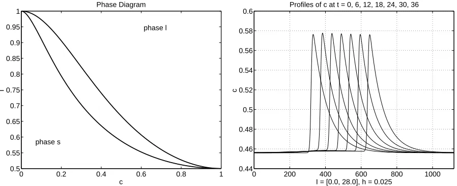
4.3. Binary isothermal systems. To model phase transformations in systems with non-trivial, non-linearized phase diagrams (see e.g. Figure 2) we need to introduce a u -dependent correction term. In this subsection we will demonstrate that our approach in fact makes it possible to obtain a superior approximation behavior also in this case.
Since ˜u = (u(1), u(2)) ∈ TΣ2 it is sufficient to consider u(1). We postulate the reduced
grand canonical potential
ψ(u(0), u(1), ϕ) = 1 2 ¡
(u(0))2+ (u(1))2¢+¡λ(u(0)−um) +G(u(1))2(3−2u(1))
¢
(1−˜h(ϕ)) with constants um = −1.0, λ = G = 0.1. The two phases l and s are in equilibrium if [ψ(u)]l
s = 0 (see Appendix A). Here, the equilibrium condition reads
u(0) =um−Gλ(u(1))2(3−2u(1)) (44)
from which we can construct the phase diagram in Figure 2 by the relations T = u−(0)1 and
c=ψ,u(1) =u(1)−6Ghs(ϕ)u(1)(1−u(1)) where hs(ϕ) := 1−˜h(ϕ). Besides we get
[c(u(1))]ls = 6Gu(1)(1−u(1)).
For the isothermal case, i.e. u(0) is constant, we solved (7) and
∂tc(u(1)) =∂tψ,u(1)(u(1)) = d∂xxu(1)
in the domainD= [0,28] for t ∈[0,40] numerically. We imposed homogeneous Neumann boundary conditions and setd= 0.4. Initially we chose foru(1) a profile as in (43) foru(0),
u(1)(0, x) =
(
u(1)∞ + (ui−u(1)∞) exp(−1dv(x−x0)), x > x0,
u(1)i , x≤x0.
(45)
Writing u(1) as a function inc we get
u(1) =
(
c, hs(ϕ) = 0,
1
12Ghs(ϕ)(6Ghs(ϕ)−1 +
p
(6Ghs(ϕ)−1)2+ 24Ghs(ϕ)c), hs(ϕ)>0.
Due to the fraction this is numerically instable as hs(ϕ) → 0. Defining β = 6Ghs(ϕ) we set u(1) =cif β ≤10−4, but checks were done with different cut off values. The following
results do not essentially depend on the cut off value.
Choosingu(1)i = 0.6 for the interface value, the equilibrium concentrations arec(l)= 0.6
and c(s) = 0.456. To model the solidification of an alloy of concentration 0.456, we let
decayc(l) andu(1) exponentially to this value by setting u(1)
∞ = 0.456. For u(1) =u(1)i = 0.6 we obtain in equilibrium u(0)eq ≈ −1.648 and an equilibrium temperature of Teq ≈ 0.6067. To make the front move we initialized with an undercooling of T = 0.55, i.e. u(0) ≡ −1
0.55.
Formula (39) yields an estimation of the initial velocity of the front: with ω0 = 0.08 we
have v ≈ ωλ0(u(0)eq −u(0))≈0.2. The initial position of the frontx0 = 8.0 was appropriately
0 0.2 0.4 0.6 0.8 1 0.5
0.55 0.6 0.65 0.7 0.75 0.8 0.85 0.9 0.95 1
c
T
Phase Diagram
phase l
phase s
0 200 400 600 800 1000
0.44 0.46 0.48 0.5 0.52 0.54 0.56 0.58
0.6 Profiles of c at t = 0, 6, 12, 18, 24, 30, 36
I = [0.0, 28.0], h = 0.025
[image:19.595.79.528.98.281.2]c
Figure 2. On the left: phase diagram for a binary mixture computed from (44). On the right: profiles of the solutioncfor the binary system in Section 4.3 during the evolution, ε = 0.4; the figure indicates already that there is only a negligible influence of the boundary conditions on the evolution as gradients ofcdon’t vanish only in the transition region. But simulations on domains with different lengths were performed to verify this conjecture.
values for ϕ again were defined as in (42). By (35), the correction term is (h and ˜h are chosen as before) ω1(u(1)) = ([c(u
(1))]l
s)2
d
H+ ˜H+J 2I .
Equation (45) does not describe the profile of a travelling wave solution, but a nearly travelling wave solution can be observed (see Figure 2). We computed the following tran-sition points ofϕ att = 20.0:
without correction with correction
ε 0.4 0√.4
2 0.2
0.2
√
2 0.4
0.4
√
2 0.2
0.2
√
2
transition 12.3923 12.3369 12.2945 12.2589 12.1928 12.1976 12.1971 12.1907 Without correction term, the changes in the interface position when changing ε are much larger than with correction term. For example, comparing the positions for ε = 0.4 and 0.2, there is a change of ≈ 10−1 without the correction term but only of ≈ 5·10−3 with.
An explicit solution to the corresponding sharp interface model to compare with is not known. But this behavior in ε indicates that the approximation of the sharp interface solution (which nevertheless should exist) is improved thanks to the correction term. A convergence rate of the interface position for the simulations with correction term could not be computed because of the oscillations in the positions (the position does not behave monotone in ε). Simulations on several slightly finer grids indicated that the numerical error is of the same size of about 10−3 which explains these oscillations.
4.4. Binary non-isothermal case. Now we will demonstrate that a better convergence behavior can also be observed if several conserved quantities are considered. We postulate the following reduced grand canonical potential:
ψ(u(0), u(1), ϕ) = 1 2 ¡
(u(0))2+ (u(1))2¢+¡λ(u(0)−um) +G(u(1)−ue)
¢
with constants um =−1.0, ue = 0.6, λ= G= 0.2. For the energy e=ψ,u(0) we postulate
the fluxK∇u(0)withK = 4.0 and for the concentrationc=ψ
,u(1) we postulated∇u(1)with
d= 0.1, i.e. there are no cross effects between mass and energy diffusion. As [c(u)]l s =G and [e(u)]l
s = λ are independent of u we obtain a constant correction term (h and ˜h are chosen as above) ω1 =
³
λ2
K + G2
d
´
H+ ˜H−2J
2I ≈ 0.8655555. Usually temperature diffusivity is much faster than mass diffusivity so that the influence of the concentration part on the correction term is much larger.
In equilibrium (see Appendix A for the conditions) we have the linear relationu(1)eq−ue =
u(0)eq −um. For u(1)=ue = 0.6 and u(0) =um =−1.0 (; T(0)=Tm = 1.0) the equilibrium concentrations are c(l) =u(1)= 0.6 andc(s)=u(1)−G= 0.4.
We solved the differential equations for x ∈ D = [0.0,1.4] and t ∈ I = [0.0,0.5] numerically. Initial values forϕ again were defined as in (42) with an interface located at
x0 = 0.6 away from the boundaries. Setting u(1)(t = 0) ≡ 0.6 and u(0)(t = 0) ≡ −1.0 we
got initial values for c and e from ψ. For ϕ and u(1) we imposed homogeneous Neumann
boundary conditions. We took the same boundary condition foru(0) inx= 1.4, but on the
other boundary point we imposed the Dirichlet boundary conditionu(0)(x= 0.0) =−1.25
which corresponds to an undercooling of 1
5 and made the transition point move to the right.
We chose ω0 = 0.08 and σ = 1.0. At t = 0.4 we measured the interface and we obtained
the following results (varying ∆x in the column and ε in the line):
∆x\ε 0.4/√2 0.2 0.2/√2 0.1 0.1/√2 with 0.002 0.704470 0.708335 0.710319
correction 0.001 0.710339 0.711441 0.712032 without 0.002 0.730569 0.726796 0.723258
correction 0.001 0.723281 0.720480 0.718347
The computations for ε = 0√.2
2 reveal that the error due to the grid is small compared
to the deviation due to the different values for ε. Computing numerically the order of convergence (see (36)) we obtained values of k ≈ 1.78 with correction term and k ≈0.57 without correction term when the runs for ε∈ {0√.4
2, 0.2
√
2, 0.1
√
2} are compared. Similar results
were obtained at the time t= 0.5.
5. Conclusions
The asymptotic analysis of a phase field model for solidification in multi-component alloy systems has been carried out using matched asymptotic expansions. In addition to the leading order problem a linear correction problem has been derived. If a certain small correction term to the kinetic coefficient in the phase field equation is taken into account the zero function solves this correction problem. Hence, there is no linear correction and our model approximates the sharp interface problem to second order.
Acknowledgement
The authors gratefully acknowledge the financial support provided by the DFG (German Research Foundation) within the priority research program (SPP) “Analysis, Modeling and Simulation of Multiscale Problems” 1095 under Grant No. Ga 695/1-2.
Appendix A. Remarks on thermodynamics
To model solidification in alloy systems, often the free energy density f is taken as thermodynamical potential. We assume that pressure and mass density are constant. Then the free energy is a function of temperature and concentrations,
f :R×ΣN →R, (T,c)7→f(T,c).
Here, T is the temperature and c = (c(1), . . . c(N)) is a vector of concentrations, i.e. c(i)
describes the concentration of component i. The free energy f is supposed to be concave inT and convex in c. Its derivative operates on the tangential space of the domain, i.e. on R×TΣN ⊂ RN+1, and its gradient can naturally be interpreted as a vector in R×TΣN, hence
Df :R×ΣN →R×TΣN, (T,c)7→Df(T,c) = (∂Tf, ∂
cf) =: (−s,µ).
The quantity s = −∂T∂ f is the entropy density and µ = ∂∂cf are generalized chemical potential differences. Written with the help of differential forms we have
df =−sdT +µ·dc.
The internal energy e is the Legendre transformed of−f with respect toT, i.e. e(s) = (−f)∗(s) =sT(s) +f(T(s)). As f is concave in T, eis concave in s. It holds
de=df +sdT +T ds=T ds+µ·dc
leading to
ds= 1
Tde−
µ
T ·dc=:−u
(0)de−u˜ ·dc.
In the following we will writee=c(0), ¯c= (c(0), c(1), . . . , c(N)) andu= (u
0,u˜). We have
−s:R×ΣN →R, ¯c7→ −s(¯c)
and assume that −s is strictly convex in ¯c. This implies already that
D(−s) :R×ΣN →R×TΣN, c¯7→ D(−s)(¯c) = u
can locally be inverted. We assume the inversion can even globally be done and that ¯ccan be written as function in u, ¯c(u) = (−Ds)−1(u). The reduced grand canonical potential
is then defined to be the Legendre transformed of −s, i.e.
ψ := (−s)∗ :R×TΣN →R, u7→ψ(u) := ¯c(u)·u+s(¯c(u)).
One would naturally identify its derivative Dψ(u) with a vector in R×TΣN. But using ¯
c(u) = (−Ds)−1(u) we can derive the derivative of ψ in u into direction v ∈ R×TΣN to be
hDψ(u),vi= d
dδ ³
(u+δv)·¯c(u+δv) +s(¯c(u+δv))´¯¯¯ δ=0
This motivates to identify Dψ(u) with ¯c(u) and to write
Dψ :R×TΣN →R×ΣN, u7→Dψ(u) = ¯c(u) = (−Ds)−1(u).
In particular, we see
d
du(0)ψ(u) =e(u),
d
du˜ψ(u) = (c
(1), . . . , c(N))(u).
One can think off,sandψ to be extended to all ofRN+1 whenever partial differentials of the functions appear. But only the definition on the domains and only derivatives in tangential direction as mentioned above will enter the equations in Sections 2, 3 and 4.
Appendix B. Transformation of derivatives near the interface
For the following computations compare also [13]. Letε0 >0. Near the interface Γ(t; 0)
we consider the diffeomorphisms
Fε(t, s, z) := (t, γ(t, s; 0) + (εz+d(t, s;ε))ν(t, s))
which, for eacht∈I andε∈(0, ε0), maps an open setV(t;ε)⊂R2onto an open tubeB(t)
around Γ(t; 0). The parameters is the arc-length of Γ(t; 0) andνand γ are as in Section 2. The coordinates (t, s, z) are such that the interface is given by the set {Fε(t, s, z)|z = 0}. It is supposed that, uniformly int, s andε, the tubeB(t) is large enough such that values forz lying in a fixed interval around zero are allowed as arguments forz. We are interested in the inverse of the derivative ofFε to obtain ∇(t,x)z(t, x) and ∇(t,x)s(t, x).
Let κ := κ(t, s; 0) be the curvature of Γ(t; 0) defined by ∂sτ = κν or, equivalently, by
∂sν=−κτ. Furthermore let
v =v(t, s; 0) =∂tγ(t, s; 0)·ν(t, s; 0) (normal velocity, intrinsic),
vτ =vτ(t, s; 0) =∂tγ(t, s; 0)·τ(t, s; 0) (tangential velocity, non intrinsic).
Hence, writingdε =d(t, s;ε) we get
DFε(t, s, z) =
µ
∂tt(t, s, z) ∂st(t, s, z) ∂zt(t, s, z)
∂tx(t, s, z) ∂sx(t, s, z) ∂zx(t, s, z)
=
µ
1 0 0
∂tγ+ (εz+dε)∂tν+ (∂tdε)ν τ −(εz +dε)κτ+ (∂sdε)ν εν
and
D(Fε−1)(t, x) = (DFε)−1(t, x) =
∂tt(t, x) ∇xt(t, x)
∂ts(t, x) ∇xs(t, x)
∂tz(t, x) ∇xz(t, x)
=
1 (0,0)
−1−κ(εz1+dε)(vτ+ (εz+dε)τ ·∂tν)
1 1−κ(εz+dε)τ
⊥
1 ε
³
−∂tdε+ ∂
sdε(εz+dε)
1−κ(εz+dε)τ ·∂tν+
∂sdε
1−κ(εz+dε)vτ −v
´ 1 εν
T − ∂sdε
ε(1−κ(εz+dε))τ ⊥
Inserting the ansatz dε = εd1(t, s) +ε2d2(t, s) +. . . we obtain for a function b(t, s, z)
and for a vector field~b(t, s, z) d
dtb = − 1
εv∂zb+∂◦b−(∂◦d1)∂zb+O(ε) ∇xb =1ε∂zb ν+ (∂sb−∂sd1∂zb)τ
+ε¡κ(z+d1)∂sb−(∂sd2+∂sd1κ(z+d1))∂zb
¢
τ+O(ε2)
∇x·~b=1ε∂z~b·ν+ (∂s~b−∂sd1∂z~b)·τ
+ε¡κ(z+d1)∂s~b−(∂sd2+∂sd1κ(z+d1))∂z~b
¢
·τ+O(ε2) ∆xb =ε12∂zzb−1εκ∂zb
+ (∂sd1)2∂zzb−2∂sd1∂szb−κ2(z+d1)∂zb−∂ssd1∂zb+∂ssb+O(ε) where ∂◦ =∂t−vτ∂s is the (intrinsic) normal-time-derivative (see e.g. [18]).
Appendix C. Expansions of interfacial normal velocity and curvature
Let us assume that the normal velocity and the curvature of Γ(t;ε) can be expanded in
ε-series, i.e.
v(t, s;ε) = v0(t, s; 0) +εv1(t, s; 0) +ε2v2(t, s; 0) +. . . ,
κ(t, s;ε) = κ0(t, s; 0) +εκ1(t, s; 0) +ε2κ2(t, s; 0) +. . . .
By (10) and the following paragraph, the interfaces Γ(t;ε) are parametrized by γε :=
γ(t, s;ε) = γ(t, s; 0) +dεν(t, s; 0) wheredε =d(t, s;ε) =εd1(t, s) +ε2d2(t, s) +. . .. We want
to identify the functions vi, κi in terms of the functions di(t, s), i= 1,2, . . ., v :=v(t, s; 0) and κ:=κ(t, s; 0).
The unit tangential vector and the unit normal vector are
τ(t, s;ε) = ∂sγε |∂sγε|
= (1−κdε)τ+ (∂sdε)ν ((1−κdε)2 + (∂sdε)2)1/2
,
ν(t, s;ε) = ∂sγε⊥ |∂sγε|
= (1−κdε)ν−(∂sdε)τ ((1−κdε)2 + (∂sdε)2)1/2
.
Inserting the expansion fordε yields
³
(1−κdε)2+ (∂sdε)2
´−1/2
= 1 +εκd1(t, s) +O(ε2)
and finally for v(t, s;ε) the expansion
v(t, s;ε) = ∂tγε·ν(t, s;ε)
= (∂tγ(t, s; 0) +∂tdεν+dε∂tν)·((1−κdε)ν−(∂sdε)τ) ((1−κdε)2+ (∂sdε)2)1/2
= (1−κdε)v+∂tdε(1−κdε)−∂sdεvτ −dε∂sdε∂tν·τ ((1−κdε)2+ (∂sdε)2)1/2
=v+ε∂◦d1+O(ε2)
where we used∂tν·ν = 12∂t|ν|2 = 0. To compute the expansion of κ(t, s;ε) we need
∂ssγ(t, s;ε) =−
³
2(∂sdε)κ+dε(∂sκ)
´
τ +³κ+∂ssdε−κ2dε
Then
det(∂sγ(t, s;ε), ∂ssγ(t, s;ε)) = −(1−κdε)(κ+∂ssdε−κ2dε)−(∂sdε)(2(∂sdε)κ+dε(∂sκ)).
As
|∂sγε|−3 = (1−2κdε+κ2d2ε + (∂sd2ε))−3/2 = 1 +ε3κd1+O(ε2)
we obtain
κ(t, s;ε) = −det(∂sγε, ∂ssγε) |∂sγε|3
=κ+ε³κ2d1+∂ssd1 ´
+O(ε2).
Appendix D. Derivation of matching conditions
In this appendix we will derive the conditions (15)-(18) foru. Analogous results can be obtained for ϕ.
By (11) and (12) the functions ˆuk(t, s, r) =uk(t, x) are well defined in the neighborhood of Γ(t; 0) which we suppose to be a tube of radiusδ0. We assume that they can smoothly
and uniformly be extended onto Γ(t; 0) from both sides as r &0 and r %0 respectively. An expansion in Taylor series inr = 0 yields
ˆ
uk(t, s, r) = ˆuk(t, s,0+) +∂ruˆk(t, s,0+)r+ 12∂rruˆk(t, s,0+)r2+O(r3), r∈(0, δ0], (46)
ˆ
uk(t, s, r) = ˆuk(t, s,0−) +∂ruˆk(t, s,0−)r+ 12∂rruˆk(t, s,0−)r2+O(r3), r∈[−δ0,0).
(47)
Letα∈(0,1) andl(t) be the length of Γ(t; 0). We assume that the expansion
ˆ
u(t, s, r;ε) = N
X
k=0
εkuˆk(t, s, r) +O(εN+1) (48)
is valid uniformly on{(t, s, r;ε) :t ∈I, s∈[0, l(t)], r∈(εα δ0
2, δ0], ε∈(0, ε0]}.
We assume that the functions Uk(t, s, z) in (13) are defined for t ∈I, s ∈ [0, l(t)] and
z ∈Rand that they approximate some polynomial in z uniformly int, s for large z, i.e.
Uk(t, s, z)≈U±k,0(t, s) +U±k,1(t, s)z+U±k,2(t, s)z2+· · ·+U±k,nk(t, s)z
nk
, z → ±∞ (49)
with nk ∈ N for all k. Besides we assume that the expansion (13) is valid uniformly on {(t, s, z;ε) :t∈I, s∈[0, l(t)], z ∈εα−1[−δ
0, δ0], ε ∈(0, ε0]}.
To derive the matching conditions let ζ ∈ (δ0
2, δ0) and ε ∈ (0, ε0] and consider the
intermediate variable ζεα. The expansion (48) is valid with r = ζεα for ε small enough. We can use (46) and get (dropping the uniform dependence on (t, s))
ˆ
u(ζεα;ε) =ε0uˆ0(0+) +εα∂ruˆ0(0+)ζ+ε2α12∂rruˆ0(0+)ζ2+O(ε3α)
+ε1uˆ1(0+) +ε1+α∂ruˆ1(0+)ζ+ε1+2α12∂rruˆ1(0+)ζ2+O(ε1+3α)
+ε2uˆ
2(0+) +ε2+α∂ruˆ2(0+)ζ+ε2+2α12∂rruˆ2(0+)ζ2+O(ε2+3α)
+O(ε3+ε4α).
Using (47) the same can be written for−ζ ∈(δ0
2, δ0) with 0
Now, for ζ positive again (13) is valid for the choice z = ζεα−1. Using (49) and again
dropping the dependence on (t, s) we obtain
U(ζεα−1;ε) =ε0U+0,0+εα−1U+0,1ζ+· · ·+εn0(α−1)U+
0,n0ζ
n0
+ε1U+1,0+ε1+α−1U1+,1ζ+· · ·+ε1+n1(α−1)U+
1,n1ζ
n1
+ε2U+2,0+ε2+α−1U2+,1ζ+· · ·+ε2+n2(α−1)U+
2,n2ζ
n2 +. . .
The same holds true for −ζ ∈(δ0
2, δ0) with U
+ replaced by U−.
The expansions of U and ˆu are said to match if, in the limit ε &0, the coefficients to every order in ε and ζ agree. Comparing the two series for U and ˆu yields the following relations between the coefficients U+k,n on the one hand and the derivatives ∂j
ruˆl(0+) on the other hand for k≤2:
U+0,0 = ˆu0(0+), U+0,i = 0, 1≤i≤n0,
U+1,0 = ˆu1(0+), U+1,1 =∂ruˆ0(0+), U+1,i = 0, 2≤i≤n1,
U+2,0 = ˆu2(0+), U+2,1 =∂ruˆ1(0+), U+2,2 = 12∂rruˆ0(0
+), U+
2,i = 0, 3≤i≤n2.
Obviously from the definition of r, a derivative of some function with respect to r corre-sponds to the derivative with respect to x into the direction ν = ν(t, s(t, x); 0). Hence, we can replace ∂ruˆk by ∇uk ·ν. As ν is independent of r we can also replace ∂rruˆk by (ν· ∇)(ν· ∇)uk. We use (49) again and obtain the following matching conditions (compare (15)-(18)): As z→ ±∞
U0(z)≈u0(0±),
U1(z)≈u1(0±) + (∇u0(0±)·ν)z,
∂zU1(z)≈ ∇u0(0±)·ν,
∂zU2(z)≈ ∇u1(0±)·ν+ ¡
(ν· ∇)(ν· ∇)u0(0±) ¢
.
References
[1] N.D. Alikakos, P. Bates, and X. Chen, Convergence of the Cahn-Hilliard equation to the Hele-Shaw model, Arch. Rational Mech. Anal. Vol. 128, No. 2, pp. 165-205 (1994).
[2] R.F. Almgren, Second-order phase field asymptotics for unequal conductivities, SIAM J. Appl. Math. Vol. 59, No. 6, pp. 2086-2107 (1999).
[3] H.W. Alt and I. Pawlow, A mathematical model of dynamics of non-isothermal phase separation, Phys. D Vol. 59, pp. 389-416 (1992).
[4] C. Andersson, Third order asymptotics of a phase-field model, TRITA-NA-0217, Dep. of Num. Anal. and Comp. Sc., Royal Inst. of Technology, Stockholm (2002).
[5] Z. Bi and R.F. Sekerka, Phase-field model of solidification of a binary alloy, Phys. A Vol. 261, pp. 95-106 (1998).
[6] J.F. Blowey and C.M. Elliott, Curvature dependent phase boundary motion and parabolic double obstacle problems. Degenerate diffusions (Minneapolis, MN, 1991), IMA Vol. Math. Appl. Vol. 47, Springer, pp. 19-60 (1993).
[7] W.J. Boettinger, S.R. Coriell, A.L. Greer, A. Karma, W. Kurz, M. Rappaz, and R. Trivedi, Solid-ification Microstructures: Recent Developments, Future Directions, Acta Mat. Vol. 48, pp. 43-70 (2000).
[8] W.J. Boettinger, J.A. Warren, C. Beckermann, and A. Karma, Phase-field simulations of solidifica-tion, Ann. Rev. Mater. Res. Vol. 32, pp. 163-194 (2002).