University of Warwick institutional repository: http://go.warwick.ac.uk/wrap
This paper is made available online in accordance with
publisher policies. Please scroll down to view the document
itself. Please refer to the repository record for this item and our
policy information available from the repository home page for
further information.
To see the final version of this paper please visit the publisher’s website
.
Access to the published version may require a subscription.
Author(s): E Riccomagno, JQ Smith and P Thwaites
Article Title: Algebraic discrete causal models
Year of publication: 2010
http://www2.warwick.ac.uk/fac/sci/statistics/crism/research/2010/paper
10-11
(will be inserted by the editor)
Algebraic discrete causal models
Eva Riccomagno · Jim Q. Smith · Peter Thwaites
Received: date / Revised: date
Abstract The main feature of the paper is to show that Algebraic Statistics is a natural framework to address issues of causality and to help discern a total cause. Indeed identifiability of an effect of a cause in discrete models is almost algebraic rather than graphical in nature. It is useful to think of it as such and it leads to the definition of a large class of discrete models which comprises popular ones.
Keywords Causality· Algebraic Statistics·Identifiability
1 Introduction
Much recent work in the field of causality has focused on how cause relates to control, and the analysis of controlled models. We assume the existence of a background idle system which is subjected to some sort of intervention or manipulation. Indeed in a common scenario, in fields such as epidemiology and economics, an observer collects data from a system and wants to make inference about what would happen were the system been controlled, for example by imposing a new treatment regime. The data generating process and hypotheses on the causal mechanism, governing both the idle system and the manipulated system, are to be specified in order to make predictions. The framework of Markov or Semi-Markovian models has been extensively adopted.
The Bayesian network has been one of the most successful graphical tools for representing complex dependency relationships and the directionality of
E. Riccomagno
Department of Mathematics, Universit`a di Genova Via Dodecaneso 35
Tel.: +39-010-5646938
E-mail: [email protected]
edges has been interpreted as causal in some way. This has led to the develop-ment of the Causal Bayesian Network, using a non-parametric representation based on structural equation models. These provide a framework for expressing assertions about what might happen when the system under study is externally manipulated and some of its variables are assigned certain values. The causal Bayesian network is often used to determine whether or not a causal effect can be deduced from non-experimental data obtained from an idle system.
Many authors have developed useful methods for defining causality and investigating its identifiability under various sampling schemes. Our main ref-erences are Pearl (2000), Spirtes et al. (1993) and Shafer (1996).
In this paper by collecting together and developing some results in the literature, we aim to illustrate how looking at the formal algebraic aspects of algebraic statistical models and of the notion of causality allows us to capture the mathematical essence of a causal statistical model and allows for a fully general modelling framework freed of the regularity constraints of Bayesian networks.
2 Algebraic set-up for causal Bayesian networks
This is a review section. The remainder of the paper generalises models and ideas presented here showing that the applicable mathematical technologies are the same as for Bayesian networks. For an ample discussion of formal mathe-matical structures for conditional independence see Studen´y (2004). Here we consider only discrete setting. Little is available in the algebraic statistics lit-erature for the continuous case. LetX= (X1, X2, ..., Xn) be a random vector where Xi takes values in the finite set Xi, for i = 1, . . . , n and the sample space forXbecomesX=ni=1Xi.
Consider a directed acyclic graph whose nodes are in one-to-one correspon-dence with the components ofX. Label the nodes compatibly with the graph, namely 1≤j < i≤n, hence Xj < Xi, whenever there is a direct path from node j to node i. This can be interpreted causally by stating that an edge fromj into icorresponds to a direct causal influence ofXj onXi.
The graph can also be taken to represent conditional independence con-straints on the components ofX, namely each variable is independent of all its non-descendants given its direct parents in the graph. This corresponds to the following factorization of a joint probabilitypforX
p(x1, . . . , xn) = n
i=1
p(xi|pai) for all (x1, . . . , xn)∈X (1)
wherep(xi|pai) is the probability ofXitaking the valuexi ∈Xigiven that its parents amongX1, . . . , Xv,v < i, take valuespai. The set of all distribution for
Xsatisfying Equations (1) gives a statistical model based on a causal Bayesian network.
the right-hand side of Equation (1). Furthermore, we focus on the problem of prediction of intervention effects. The simplest kind of intervention, which we call atomic intervention, is as follows. Thejth component of Xj is forced to take a specific value, say ˆxj∈Xj, with probability one and a new density, or post-intervention density, is defined on{X1, . . . , Xn} \ {Xj} by the recursive formula
p(x1, . . . , xj−1, xj+1, . . . , xn||xˆj) = n
i=1,i=j
p(xi|pai) (2)
with p(xi|pai) as above, but noting that if Xj is a parent of Xi then the component ofpai corresponding toXj takes the value ˆxj. Equation (2) corre-sponds to a sub-graph obtained by removing the nodejtogether with its edges. Successive atomic interventions of this type produce an atomic intervention on a subset of{X1, . . . , Xn}.
The pre-intervention and post-intervention densities can be combined in a single framework by adding an extra nodej and an extra edge fromjin j. The new node corresponds to a random variableFjtaking values inXj∪{idle}. A joint probability on the augmented causal graph is defined as
p(x1, . . . , xn, fj) =
⎧ ⎨ ⎩
p(x1, . . . , xn) iffj =idle
p(x1, . . . , xj−1, xj+1, . . . , xn||xˆj) iffj = ˆxj
0 otherwise
(3)
Often it is of interest to estimate the post-intervention distribution, some of its marginal or some other functions, from non-observational data from the pre-intervention distribution. Each factor in the right hand side of Equa-tion (1) can be interpreted as a data simulator, or data generating process. At a structural level, we could ask whether some functioneof the post-intervention distribution can be explicitly written as a function of the variables appearing in Equation (1) either on the right hand side or left hand side. Clearly, this is possible for anyeif all values ofXare observables prior intervention. But, if there are unobservable or hidden variables in the model, the questions is more difficult and the answer depends on the modular structure imposed by the graph on the model, on the structure of the observed, or manifest, variables, and on the intervention and importantly on how these three are related. We shall go back to this in Section 4.
2.1 Algebraic representation of (causal) Bayesian networks
Consider a simple example. For X1, X2, X3 binary with levels 1−2, the graphX1→X2→X3and the atomic intervention ˆx2= 1, Equations (1) are
p(x1, x2, x3) =p(x1)p(x2|x1)p(x3|x2), forx1, x2, x3∈ {1,2} (4)
and Equations (2) become
p(x1, x3||xˆ2) =p(x1)p(x3|xˆ2), forx1, x3∈ {1,2}
It can be shown that the first set of equations is satisfied by any function on
{1,2}3taking non-negative values summing to one and satisfying the following two polynomial equations
−p(1,2,2)p(2,2,1) +p(1,2,1)p(2,2,2) = 0 (5)
−p(1,1,2)p(2,1,1) +p(1,1,1)p(2,1,2) = 0 (6)
The polynomials in the right hand side of (5) above can be taken to provide an implicit description of the graphical modelX1→X2→X3. These are ob-tained by eliminating the conditional probabilities from Equations (4) and are generators of the set of all polynomials which are invariant under the model. Analogously, the polynomial invariants of the manipulated graph, expressed in the joint probabilities, are of the form af with f = p(1,1,2)p(2,1,1)− p(1,1,1)p(2,1,2) and a any polynomial in the p(x1, x2, x3), (x1, x2, x3) ∈ {1,2}3.
Together with the polynomial constraints in (4) imposed by the condi-tional independence model, there are other obvious algebraic constraints like
x1,x2,x3p(x1, x2, x3) = 1 in the joint probabilities and
x2p(x2|x1)−1 in
the conditional probabilities and there are some inequalities such as the non-negativity of probabilities which render the set of probability densities satis-fying the modelX1→X2→X3 a semi-algebraic set, namely a space defined
by polynomial identities and inequalities.
The theory behind the elimination process that leads to the implicit de-scription of Bayesian networks is a branch of Algebraic Geometry called Elimi-nation Theory (Cox et al. (2008)). It is fairly well understood and implemented in general computer algebra software such as Maple and Matlab. However, its use in applied contexts may be limited by the fact that actual computations are often unfeasible and more refined ways to eliminate are to be sought. For Bayesian networks with and without hidden variables, Garcia, Stillman, and Sturmfels (2005) study the algebraic varieties defined, in particular they show that the naive Bayes model corresponds to the higher secant varieties of Segre varieties.
To handle the semi-algebraic aspects, Drton and Sullivant (2007) use the Tarski-Seidenberg theorem on projections to show that the (well-defined) im-age of a semi-algebraic set through the rational map defined by Equations (1) on the simplex is still semi-algebraic.
together with more standard topological arguments. Typical topological iden-tifiability theorems are the back door and front door criteria for ideniden-tifiability of a cause of an effect. The set of variables is now augmented to comprise also variables expressing the polynomial equalities and inequalities for the ob-served (or observable) functions. If in the simple example above we observe the joint probability of X2 and X3 then we would have four more variables
m(x2, x3) =p(1, x2, x3) +p(2, x2, x3),x2, x3∈ {1,2}2.
In computational biology, several authors including Allman, Rhodes and co-workers (2003, 2008) use the algebraic representations of Markov models to address identifiability issues within the field of molecular phylogenetics where it is of interest to infer evolutionary trees from DNA or protein sequences. Identification problems associated with the estimation of some probabilities after manipulation from passive observations (manifest variables measured in the idle system) have been formulated as an elimination problem in computa-tional commutative algebra, for example in the case of Bayesian network the case study in Kuroki (2007). In general, a systematic implementation of these problems in computer algebra softwares will be slow to run. At times some pre-processing can be performed in order to exploit the symmetries and invari-ances to various group action for certain classes of statistical models (Mond et. al (2003)). Other times a re-parametrisation in terms of non-central moments loses an order of magnitude effect on the speed of computation and hence can be useful (e.g. Settimi and Smith (2000) and Zwiernik and Smith (2009)).
In Algebraic Statistics, the identifiability of causal effects for causal Bayesian networks with hidden variables is addressed by Kang and Tian (2007) via the notion of c-component (Tian and Pearl (2002)). They provide an algorithm to determine polynomial constraints that a causal Bayesian network must sat-isfy “to be compatible with given observational and experimental data”. In the algebraic framework of this paper many non-graphically based symmetries which appear in common models are much easier to exploit than in a solely graphical setting. This suggests that the algebraic representation of causality is a promising way of computing the identifiability of a causal effect in much wider classes of models than Bayesian network.
3 Generalisations
Wider classes of discrete statistical models than causal Bayesian networks have an analogous algebraic formulation. These can overcome symmetry restrictions implied by the requirement of a product sample space in a Bayesian network and allow a larger class of manipulations. In this section, we present a point summary for causal Bayesian networks and define some of these wider classes by generalising one or more of those items.
2. a discrete Bayesian network can be described through a set of linear equa-tions together with inequalities to express non negativity of probabilities and linear equations for the sum-to-one constraints. Namely, for all i = 1, . . . , nsetp(xi|x1, . . . , xi−1) =p(xi|x1, . . . , xi−1) whenever (x1, . . . , xi−1)
and (x1, . . . , xi−1) coincide on the parent set ofXi(see Dawid and Studeny (1999)). We refer to this as the transition or primitive probabilities; 3. a Bayesian network is based on the assumption that the factorization in
Equation (1) holds across all values ofxin a cross product sample space. But in Settimi and Smith (2000) it is shown that identification depends on the sample space structure, in particular on the number of levels a variable takes;
4. within a graphical framework subsets of whole variables inX are consid-ered manifest or hidden;
5. mainly the causal controls being studied in e.g. Pearl (2000); Spirtes et al. (1993) correspond to setting subsets of variables in X to take particular values and often the effect of a cause is expressed as a polynomial function of the primitive probabilities, for example marginals;
6. identification problems are basically elimination problems and can be ad-dressed using elimination theory from computational commutative algebra coupled with a pre-processing based e.g. on topological arguments.
3.1 Bayesian linear models
A Bayesian network can defined through linear constraints on some conditional probabilities according to an ordering of the nodes compatible with the graph, see Item 2 above. A Bayesian linear constraint model (Riccomagno and Smith (2004)) is a straightforward generalisation given by 1. a total order on the components of X and an associated collection of factorisation formulae like Equations (1); 2. a set of linear equations in transition probabilities
Li(p(xi|x1, . . . , xi−1) =
xi∈Xi
axi,x1,...,xi−1p(xi|x1, . . . , xi−1) = 0
with real coefficientsaxi,x1,...,xi−1; 3. a set of linear inequalities with real
coef-ficients on the transition probabilities of the form
Li(p(xi|x1, . . . , xi−1))≤Mi(p(xi|x1, . . . , xi−1)).
A Bayesian linear constraint model is called feasible if there is at least a prob-ability distribution over the sample space X satisfying 1-3 above. Again the Tarski-Seidenberg can be invoked to guarantee that Bayesian linear constraint model are algebraic models.
especially for large sample size where some variables in the network have a dis-tribution conditional on their parents which is parametric and the transition probabilities are a (rational) polynomial function of the distribution parame-ters, for example a Binomial distribution with a known number of independent trials and unknown success probability; and finally chain graph models.
Intervention is defined for a feasible Bayesian linear constraint model as in a Bayesian network by forcing some variables to assume given values and the post intervention distribution is expressed by equations resembling Equa-tions (2). Again the post intervention distribution needs to continue to respect the equality and inequality constraints in 2-3 above.
3.2 Tree based generalization
For a probability treeT with vertex set V and edge set E and for v, v ∈V, (v, v) ∈ E, let π(v|v) be the possibly unknown transition probability from v to v, under the constraint v:(v,v)∈Eπ(v|v) = 1. The values π(v|v), (v, v)∈ E, parametrize the model and are the primitive or transition prob-abilities. The probability of the event corresponding to the root-to-leaf paths λ= (v0, . . . , vn(λ)), where v0is the root vertex and vn(λ)a leaf vertex is
p(λ) = n(λ)−1
i=0
π(vi+1|vi) see Equation (1) (7)
The nodes of the tree and the root-to-leaf paths, which are analogue to the joint probabilities for Bayesian networks, are the topological keys to the two parametrisations.
There is a natural partial order associated with the tree which can be used as a framework to express causality. If in the tree the event expressed by nodev occurs before the one represented byv wheneverv≺v, then the effects of a control on a regular tree T can now be defined in total analogy to Item 5 above by modifying the values of some primitive probabilities or more generally by defining constraints in the primitive probabilities that have a causal interpretation. Hence a manipulation of the tree is given by a subset F ⊂Eand new transition probabilities ˆπon the edges inFwhich are functions of the primitive probabilities and compatible with the existing model.
3.3 Extreme causality
Note that to discuss causal maps we need 1. a finite set of controllable “cir-cumstances” and a finite set of outcomes of an experiment, and 2. a partial order defined on these circumstances, more abstractly 1. a finite setV ={v} and 2. a partial order onV,≺. A chain of the Hasse diagram of the ordering
≺represents a possible unfolding of the experiment. The structure is that of a directed acyclic graph, like in a Bayesian network, but where each node stands for an event, like in a probability tree.
A saturated statistical model onV can be defined giving a set of transition probabilities:π(v|v)∈[0,1] where v, v ∈V are in the same chain and there is nov∗in the chain such thatv≺v∗≺v.
The probability of a chainλ= (v0, . . . , vn(λ)) isp(λ) =in=1(λ)π(vi|vi−1) (cf.
Equation (1)). The sum to one condition holds and states thatvπ(v|v) = 1. An algebraic sub-model is defined by setting to zero suitable algebraic equa-tions of the transition probabilities and by imposing some polynomial inequal-ities among them.
A manipulation or control can now be defined implicitly by considering a setFof edges of the Hasse diagram and assigning to (v, v)∈Fa new primitive probabilityπ(v|v) which we take to be a polynomial function of the vector of primitive probabilitiesπ’s. This could be of the atomic type by setting to one someπ(·|·), or more generally, and often realistic, simply another probability densities on the Hasse diagram
3.4 An example
Consider a statistical model built to study whether watching a violent movie might induce a man into a fight, allowing for testosterone levels to, at least partially, explain a violent behaviour. This could be modelled with a Bayesian network. Let X2 denote whether a man watches a violent movie early one
evening{x2= 1}or not{x2= 2}and letX4 be an indicator of whether he is
arrested for fighting{x4= 1}or not{x4= 2}late that evening. If he watches
the movie, letX1 denote his testosterone level just before seeing it andX3his testosterone level late that evening. For a man who does not watch the movie letX1=X3 denote his testosterone level that evening.
Assume X1 and X3 take three values: 1 for low levels of testosterone, 2 for medium levels and 3 for high levels, so that (r1, r2, r3, r4) = (3,2,3,2) and r= 36. Then this can be depicted as the following Bayesian example
X1→X3 ↓
X2→X4
one states that the testosterone level before watching the movie gives no ad-ditional relevant information about the man’s inclination to violence provided that we happen to know both whether he watched the movie and his current testosterone levels.
There are 36 elements in the sample space X and a general joint mass function on (X1, X2, X3, X4) is given by the 36 quartic equations
p(x) =π1(x1)π2(x2|x1)π3(x3|x1, x2)π4(x4|x1, x2, x3). (8)
The conditional independence statements in Item 2 are given by
π2(x2|x1) =π2(x2|x1)π2(x2) (say) (9)
π4(x4|x1, x2, x3) =π4(x4|x1, x2, x3)π4(x4|x2, x3) (say)
for all x1, x1 = 1,2,3. The simple substitution of Equations (9) into (8)
allows us to reduces the number of parameters and of constraints. Indeed the resulting vectors (π1(1), π1(2), π1(3)) lie in three-dimensional simplex Δ2
as do each of the vectors (π3(1|x1, x2), π3(2|x1, x2), π3(3|x1, x2)) for x1 = 1,2,3 and x2 = 1,2 whilst the vectors (π2(1), π2(2)) and each of the vec-tors (π4(1|x2, x3), π4(2|x2, x3)) for x2 = 1,2 andx3 = 1,2,3 lies inΔ1. Each of the 14 simplices also embodies a linear constraint through its sum-to-one condition making the interior of the domain a 21 dimensional linear manifold. Now, other non-graphical hypotheses are added to the condition indepen-dence statements expressed by the Bayesian network. The new hypotheses can still be expressed as a set of algebraic equations or inequalities on the primitive probabilities. We list some for our example.
– If the movie is not watched then we would expect X3 = X1|(X2 = 2), equivalently
π3(x3|x1, x2= 2) =
1 ifx3=x1
0 otherwise. (10)
– If a unit did watch the movie, we would not expect this to reduce his testosterone level. This sets some of the primitive probabilities to zero, namely
X3|X1=x1, X2= 1 x3= 1 x3= 2 x3= 3
x1= 1 π3(1|1,1)π3(2|1,1)π3(3|1,1)
x1= 2 0 π3(2|2,1)π3(3|2,1)
x1= 3 0 0 1
(11)
– The assumption that the higher the prior testosterone levels the higher the posterior ones, is given by
π3(1|2,1) =r3,2π3(1|1,1) (12) π3(3|1,1) =r3,3π3(3|2,1)
– Similarly it is reasonable to expect that higher levels of testosterone to-gether with having seen the movie would make more probable that a man would be arrested for fighting. This can be expressed as
π4(1|1, x3) =r4,x3π4(1|2, x3) forx3= 1,2,3
π4(1|1, x3+ 1) =r4,x3π3(1|1, x3) forx3= 1,2
π4(1|2, x3+ 1) =r4,x3π3(1|2, x3)
where 0≤r4,x3, r4,x3, r4,x3≤1, similarly to the previous bullet point. – Finally a common simple log-linear response model might assumer4,1 =
r4,2=r4,3.
The point here is not that these supplementary equations and inequalities pro-vide the most compelling model, but rather that embellishments of this type, whilst not graphical, are common, are easily expressed in the primitive prob-ability parametrization, and often have an almost identical type of algebraic description as the Bayesian example.
4 (Algebraic) identifiability
Identifiability problems are formulated in the classes of models in Section 3 in the same way. Some polynomial equalities of the transition probabilities, say m = m(π), are observed or observable together with some inequalities. The interest is in checking whether a total cause (Pearl (2000)) expressed as a function of the post intervention transition probabilities, saye=e(π), can be written as functions of them’s.
In principle this computation can be done by using elimination techniques from algebraic geometry but, usually, this is not feasible in practice, even less so than in Bayesian networks. If an effecteis identifiable then it is a ratio of polynomials in the observable variables by the Tarski-Seidenberg theorem and could be found by a powerful enough computer.
4.1 Non-regular observables and effects
With refer to the example in Section 3.4 we show that sometimes the mani-fest/hidden variables are not full marginal, but are rather some (polynomial) function of transition probabilities. Likewise the causal effect that it is neces-sary to identify might be not a full marginal. Hence an algebraic model of the type discussed in this paper might be appropriate.
Consider collecting data whenX4is hidden and it is the variable of central
interest with its associated probabilitiesπ4(x4|x1, x2, x3). It might be possible
to randomly sample men and measure their testosterone levels before and after watching a violent movie. Call this Experiment 1. However if it were believed that watching a violent movie might induce a fight, it would be unethical to release the subjects after watching the movie, while any therapy either in the form of drugs or counselling will corrupt the experiment. In any case record-ing the proportions of subjects who later fought would not give an appropriate estimate of probabilities associated withX4and conditional on its parents. So values likeπ4(2|x1,1, x3) cannot be estimated from such samples. To identify the system we therefore need to supplement this type of experiment with an-other measuring “willingness to fight”. Other experiments might be envisaged leading to analogues problems.
Partial information about the joint distribution ofX4with other variables
might be obtained from a random sample of men arrested for fighting{x4= 1}.
Their current testosterone levelsX3and whether they had recently watched a
violent movie X2 could be measured. But we could not measure (X2, X3) for
men that are not caught fighting. Thus the finest partition of probabilities we could hope for in a population under this kind of survey is based on the sample space partition{A, A(x2, x3}:x2= 1,2, x3= 1,2,3}whereA={x:X4= 2}
and A(x2, x3) = {x : X2 = x2, X3 = x3, X4 = 1} i.e. q(A) = xi∈Ap(x) and forx2= 1,2 andx3= 1,2,3, q(A(x2, x3)) =xi∈A(x2,x3)p(x). Call this Experiment 2.
In the example the partial order on the nodes of the Bayesian example is X1, X2 ≺X3 and X1, X2, X3 ≺ X4. But note that, in our statement of the problem, if the man does not watch the movie then by definition X1 =X3.
Under this definition, manipulatingX3and leavingX1unaffected, as would be
required by the causal Bayesian network, is not possible. If we follow the two different types of unfoldings of history:{prior testosterone level X1 = 1,2,3,
watch movie,X2= 1 posterior testosterone levelX3 = 1,2,3, arrested X4 =
1,2} and {prior testosterone level X1 = 1,2,3, don’t watch movie, X2 = 2,
arrestedX4= 1,2}this sort of ambiguity disappears and we could reasonably
conjecture that these unfoldings are consistent with their “causal order”. This might be expressed by the two context specific graphs below
X1 →X3 X1
↓
The joint mass function is no longer defined on the product spaceSXwithX =
{X1, X2, X3, X4}. However the joint mass function of each of these possible unfoldings is well defined and furthermore each unfolding is expressible as a monomial in the primitive probabilities.
5 Chain Event Graphs
Chain Event Graphs are statistical models based on a probability tree, which can have more topological structure than the model classes in Section 3 and still allow a similar algebraic set-up. They are defined through two equivalence relationships on the nodes of a probability tree,T.
Two non-leaf verticesv, v∗ofT are stage equivalent if there is a one-to-one map between the primitive probabilities on the two sets of edges out of the two vertices. They are position equivalent if 1. the two sub-trees rooted atv and v∗,T(v) andT(v∗), have the same support/tree structure (callμ this map) and 2. for every non-leaf vertexw∈ T(v),wandμ(w) are in the same stage. The chain event graph of a probability tree is a mixed graph whose vertex set is the set of positions union a sink node, whose undirected edges join positions in the same stage and whose directed edges are of two types. Namely, for each edge (v, v∗) in the tree, with v in position w, ifv∗ is in positionw∗ then add a directed edge from w to w∗ and if v∗ is a leaf node then add a directed edge fromwto the sink node.
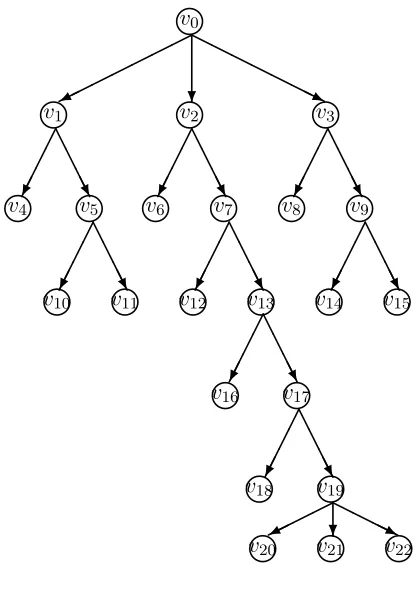
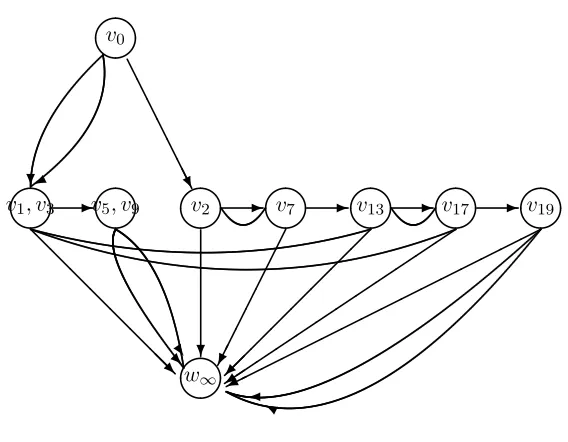
Figure 1 gives a probability tree with thirteen root-to-leaf path. The stage equivalence classes are {v1, v3, v13, v17}, {v5, v9} and {v2, v7} leading to the chain event graph with eight position nodes in Figure 2.
Anderson and Smith (2005) discuss conditional independence for Chain Event Graphs and an application to the study of biological regulation models. Propagation of probabilities over chain event graphss has been discussed in Thwaites et al. (2008) and conjugate estimation in Riccomagno and Smith (2005).
6 Manipulations
A manipulation of a probability tree is called positioned (staged) if the set of positions (stages) after manipulation is equal to or a coarsening of the set of positions (stages) before manipulation. Positioned manipulations are those that can be enacted directly on the chain event graphs.
Standard manipulation of a Bayesian network force some components of the network to take preassigned values. The analogue for a chain event graph is a manipulation which forces all paths to pass through a specified set of positionsW. E.g. assign patients with particular values of a set of covariates (their current positions) to a particular treatment regime (a set of subsequent positionsW).
l
v
0 ? HH HH HHHj lv
1v
l2v
l3A A AAU A A AAU A A AAU l
v
4v
l5v
l6v
l7v
l8v
l9A A AAU A A AAU A A AAU l
v
10v
11lv
12lv
13lv
14lv
15lA A AAU l
v
16v
17lA A AAU l
v
18v
19l
?HHHHj
l
v
20v
21lv
22lFig. 1 A probability tree
paper to show how fairly intricated topological arguments lead to a simple elimination formula for the estimation of a causal effect. It works because of how manipulation, observables and effects are defined relative to each other.
7 A back door criterion for chain event graphs
[image:14.612.103.310.82.377.2]
w
∞
v
1, v
3
v
5, v
9
v
2v
7v
13v
17v
19v
0 A A A A A AAU ? - - - - -@ @ @ @ @ @@@R ? + R^ Y
Fig. 2 A chain event graph
the directed paths in the chain event graphs through w, equivalently paths in the tree through nodes in the equivalence class w; finally let π(Λ(w)) be probability ofΛ(w).
The set W is called simple if 1. no two positions of W lie on the same directed path of the chain event graphs, 2. forw∈W π(Λ(w)) =A(w)B(w) where A(w) is a function of a set Ka ⊂ K(C∗(W)) and B(w) of Kb = K(C∗(W))\Ka and 3. A(w) is constant for w ∈ W (a stands for active, bfor background).
A manipulation is called forced to W if 1. it assigns probability one to passing throughW and 2. it leaves unchanged the probabilities on edges down-stream ofw. A manipulation is called amenable forced toW if 1.W is simple in the idle chain event graphs, 2.W is simple in the manipulated chain event graphs and the manipulation assigns probability one to passing through W, and 3. the manipulation changes only the probability of edges inKa.
[image:15.612.109.393.69.290.2]Let Z (a back door variable) be a random variable on the chain event graphs. A set of positions W is called simple conditioned on Z if 1. no two positions of W lie on the same directed path of the chain event graphs, 2. W =z:Z=zWzandWzis simple inC(Λz)1, and 3. there is a (directed) path from each wz ∈Λz through a w2 ∈ W and Wz is the set of precisely those positions inW which lie on a root-to-sink path includingwz.
Given a random variable ˆY (an effect) on a chain event graphs after a manipulation forced tow[W], it is possible to construct a random variableY on the idle chain event graphs that coincides with ˆY on the paths throughw [W].
7.1 Back door theorem
If a set W is simple conditioned on Z then the distribution of an effect ran-dom variable Y after an amenable manipulation to W is identified from the probabilities (in the idle system) of the event{Y =y, W, Z=z:y, z}, namely
ˆ
π( ˆY =y) = z:Z=z
π(Y =y, W|Z=z)
π(W|Z=z) π(Z =z)
equivalently
ˆ π(Λy) =
z:Z=z
π(Λy|Λ(W), Λz)π(Λz).
7.2 Identifying effects algebraically
We end this paper by a short discussion of how the identifiablity issues asso-ciated with the non-graphical example of Section 3.4 can be addressed alge-braically.
For the example in Section 3.4 assume conditions (10) and (11) hold. Hence, for x1 = 1,2,3 the non-zero probabilities associated with not
view-ing the movie arep(x1,2, x1,1) =π1(x1)π2(2)π4(1|2, x1) andp(x1,2, x1,2) =
π1(x1)π2(2)π4(2|2, x1) whilst the probabilities associated with viewing it are
given in Table 1.
Consider the two controls described in Section 4.1, manipulating X2 =
2 and X1 = X3 = 1 respectively. The first, banning the film, gives
non-zero probabilities for x1 = 1,2,3 satisfying the equations p(x1,2, x1,1) =
π1(x1)π4(1|2, x1) andp(x1,2, x1,2) =π1(x1))π4(2|2, x1). The second, the
fix-ing of testosterone levels to low for all time, gives manipulated probabilities
p(1,2,1,1) =π2(2)π4(1|2,1) p(1,2,1,2) =π2(2)π4(2|2,1)
p(1,1,1,1) =π1(1)π2(1)π3(1|1,1)π4(1|1,1)
p(1,1,1,2) =π1(1)π2(1)π3(1|1,1)π4(2|1,1)
p(1,1,2,1) =π1(1)π2(1)π3(2|1,1)π4(1|1,2)
p(1,1,2,2) =π1(1)π2(1)π3(2|1,1)π4(2|1,2)
p(1,1,3,1) =π1(1)π2(1)π3(3|1,1)π4(1|1,3)
p(1,1,3,2) =π1(1)π2(1)π3(3|1,1)π4(2|1,3)
p(2,1,2,1) =π1(2)π2(1)π3(2|2,1)π4(1|1,2)
p(2,1,2,2) =π1(2)π2(1)π3(2|2,1)π4(2|1,2)
p(2,1,3,1) =π1(2)π2(1)π3(3|2,1)π4(1|1,3)
p(2,1,3,2) =π1(2)π2(1)π3(3|2,1)π4(2|1,3)
p(3,1,3,1) =π1(3)π2(1)π4(1|1,3)
p(3,1,3,2) =π1(3)π2(1)π4(2|1,3)
Table 1 Probabilities associated with viewing the movie
Now consider three experiments. Experiment 1 of Section 4.1 exposes men to the movie, measuring their testosterone levels before and after viewing the film. This obviously provides us with estimates ofπ1(x1), forx1= 1,2,3 and π3(x3|1, x1) 1 ≤ x1 ≤ x3 ≤ 3. Under Experiment 2 of Section 4.1 a large
random large sample is taken over the relevant population providing good estimates of the probability of the margin of each pair of X2 and the level
of testosterone X3 on those who fought,{X4 = 1}, but only the probability
of not fighting otherwise. So you can estimate the values of and sample for x1= 1,2,3p(x1,2, x1,1) =π1(x1)π2(2)π4(1|2, x1) and
p(1,1,1,1) =π1(1)π2(1)π3(1|1,1)π4(1|1,1) p(1,1,2,1) =π1(1)π2(1)π3(2|1,1)π4(1|1,2)
p(1,1,3,1) =π1(1)π2(1)π3(3|1,1)π4(1|1,3) p(2,1,2,1) =π1(2)π2(1)π3(2|2,1)π4(1|1,2)
p(2,1,3,1) =π1(2)π2(1)π3(3|2,1)π4(1|1,3)
p(3,1,3,1) =π1(3)π2(1)π4(1|1,3).
Note the last probability is redundant since it is one minus the sum of those given above. Finally Experiment 3 is a survey that informs us about the pro-portion of people watching the movie on any night, i.e tells us (π2(1), π2(2)).
Now suppose we are interested in the total cause
e=
x1,x3
p(x1,2, x3,1) =
x1
π1(x1)π4(1|2, x1)
of fighting if forced not to watch. Clearly this is identified from an experiment that includes Experiments 2 and 3 by summing and division byπ2(2), but by no
1
2
3
1
2
1
2
1
2
1|11
2|11
3|11
1|12
2|21 3|21
2|22 3|3
1
3|32
1|11
etc
X1 X2 X3 X4
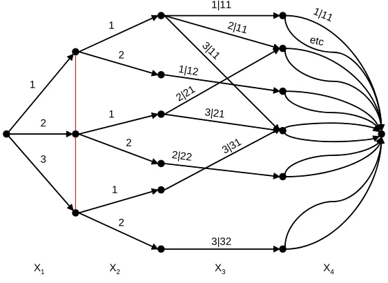
Fig. 3 Chain even graph for the movie example
fights, is identified from p(1,1,1,1) obtained from Experiment 1 and 2 by division.
The chain event graph in Figure 3 illustrate the asymmetries in our movie example and can also portray the possible manipulations. For example the manipulation which setsX2= 2 simply prunes all the edges that appear only
on (X2 = 1)-consistent paths, and assigns a probability of one to (X2 = 2)
edges. The resultant graph is of course consistent with the ˆpexpressions above. Similarly, the manipulation which setsX1 =X3 = 1 is easily represented by
pruning appropriate edges, and givesˆˆpexpressions consistent with those above.
8 Comments
[image:18.612.83.364.56.261.2](Smith and Anderson (2008)). On the other hand algebraic type of symmetries might be easily spotted and be exploited in the relevant computations.
In this example computation was simple algebraic operation while in more complex case we might need to recur to a computer. Of course the usual difficulties of using current computer code for elimination problems of this kind remain, because inequality constraints are not currently integrated into software and because of the high number of primitive probabilities involved. The advantages of ad-hoc parametrizations apply to these structures based on trees and/or defined algebraically.
References
Allman, E. S. and Rhodes, J. A. (2003). Phylogenetic invariants for the general Markov model of sequence mutation. Math. Biosci. 186, no. 2, 113–144.
Allman, E. S., An´e, C., Rhodes, J. A. (2008). Identifiability of a Markovian model of molec-ular evolution with gamma-distributed rates. Adv. in Appl. Probab. 40, no. 1, 229–249. Anderson, P.E., Smith, J.Q. (2005). A graphical framework for representing the semantics
of asymmetric models. Technical report 05-12, CRiSM.
Cox, D., Little, J. & OShea, D. (2008).Ideals, Varieties, and Algorithms 3edn. Springer-Verlag, New York.
awid, A.P. (2002). Influence diagrams for causal modelling and inference. International Statistical Review, 70, 161–189.
Dawid, A.P., Studen´y, M. (1999). Conditional products: an alternative approach to condi-tional independence. In D. Heckerman, J. Whittaker (Eds.),Artificial Intelligence and Statistics 99(pp. 32–40) Morgan Kaufmann Publishers, S. Francisco.
Drton, M., Sullivant, S. (2007). Algebraic statistical models. Statist. Sinica 17 (2007), no. 4, 1273–1297.
Garcia, L. D., Stillman, M., Sturmfels, B. (2005). Algebraic geometry of Bayesian networks. J. Symbolic Comput. 39, no. 3-4, 331–355.
Glymour, D., Cooper, G.F. (1999).Computation, Causation, and Discovery. MIT Press, Cambridge.
Hausman, D. (1998).Causal asymmetries. Cambridge University Press, Cambridge. Kang, C., Tian, J. (2007). Polynomial Constraints in Causal Bayesian Networks. In
Pro-ceedings of the Conference on UAI(pp. 200–208), AUAI Press.
M. Kuroki,Graphical identifiability criteria for causal effects in studies with an unobserved treatment/response variable, Biometrika94(1) 37–47, 2007.
Lauritzen, S. (2000). Graphical models for causal inference. In O.E. Barndorff-Nielsen, D. Cox, and C. Kluppelberg (Eds.),Complex Stochastic Systems(pp. 67–112), Chapman and Hall/CRC Press, London.
McAllester, D., Collins, M., Periera, F. (2004). Case factor diagrams for structured prob-abilistic modeling. InProceedings of the 20th Conference on Uncertainty in Artificial Intelligence(pp. 382–391), AUAI Press.
D.M.Q. Mond, J.Q. Smith and D. Van Straten,Stochastic factorisations, sandwiched simplices and the topology of the space of explanations, Proc. R. Soc. London. A459: 2821-2845, 2003.
Pearl, J. (2000).Causality: Models, Reasoning and Inference. Cambridge University Press, Cambridge.
Riccomagno, E., Smith, J.Q. (2009). The geometry of causal probability trees that are alge-braically constrained. In L. Pronzato and A. A. Zhigljavsky (Eds.),Search for Optimality in Design and Statistics(pp. 133–154), Springer-Verlag, Berlin.
Riccomagno, E., Smith, J.Q. (2004). Identifying a cause in models which are not simple Bayesian networks. InIPMU 2004(pp. 1315–1322).
Riccomagno, E., Smith, J.Q., Thwaites, P.A. (submitted). Causal analysis with chain event graphs.
Robins, J.M. (1997). Causal inference from complex longitudinal data. In M. Berkane (Ed.),
Latent variable modeling and applications to causality(pp. 69–117), Springer, New York. R. Settimi and J.Q. Smith,Geometry, moments and conditional independence trees with
hidden variables, The Annals of Statistics,28(4):1179-1205, 2000. Shafer, G. (1996).The Art of Casual ConjectureMIT Press.
Smith, J.Q., Anderson, P.E. (2008). Conditional independence and Chain Event Graphs.
Artificial Intelligence, 172, 42–68.
Spirtes, P., Glymour, C., Scheines, R. (1993).Causation, Prediction, and Search. Springer-Verlag, New York.
Studen´y, M. (2004). Probabilistic Conditional Independence Structures. Springer-Verlag, London.
Thwaites, P.A., Smith, J.Q., Cowell, R.G. (2008). Propagation using Chain event graphs. InProceedings of the 24th Conference on UAI, Helsinki.
Tian, J., Pearl, J. (2002). On the testable implications of causal models with hidden vari-ables. In Proceedings of UAI 2002, pp.567–573.