Learning and predicting with chain event graphs

(1)

University of Warwick institutional repository: http://go.warwick.ac.uk/wrap

A Thesis Submitted for the Degree of PhD at the University of Warwick

http://go.warwick.ac.uk/wrap/4529

This thesis is made available online and is protected by original copyright.

Please scroll down to view the document itself.

(2)

M A

E

G

NS I

T A T MOLEM

U N

IV ER

SITAS WARWICEN

SIS

Learning and Predicting with Chain Event Graphs

by

Guy Freeman

Thesis

Submitted to the University of Warwick

for the degree of

Doctor of Philosophy

Department of Statistics

(3)

List of Tables

6.1 Selected stages of MAP CEG model found from data described in Section 6.1.2 using AHC. The columns respectively detail the stage number, posterior expectation of the probability vector of that stage (rounded to two decimal places), number of students passing through that stage in the dataset, number of situations from the original ET in that stage, examples of situations in that stage (shown as sequence of achieved grades 1, 2 or 3, and where 4 means that the grade is missing), and any comments or observations related to that stage. . 103 6.2 All possible stagings and their posterior probabilities at each time

t for k = 0.9, ρ = 0.9, q = 0.2 with P(C1 = {v1, v2, _{v3, . . . , v6},

(7)

List of Figures

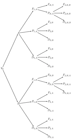
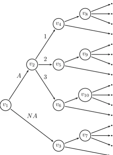
1.1 Event tree of a student’s potential progress through a hypotheti-cal course described in Example 1. Each non-leaf node represents a juncture at which a random event will take place, with the selec-tion of possible outcomes represented by the edges emanating from that node. Each edge distribution is deﬁned conditional on the path passed through earlier in the tree to reach the speciﬁc node. . . 4 1.2 Event tree for marks for two modules in a course. Marks are

dis-cretized into 3 grades, and A and N A indicate whether the mark is recorded or missing. The 10 situations are labelled and the 16 leaf nodes are unlabelled. . . 8

3.1 Floret ofv. This subtree represents both the random variable X(v)

and its state spaceX(v). . . 32 3.2 Simple event tree. The non-zero-probability events in the joint

prob-ability distribution of two Bernoulli random variables,AandB, with

(8)

3.4 Event tree for idle and manipulated versions of the same process . . 37

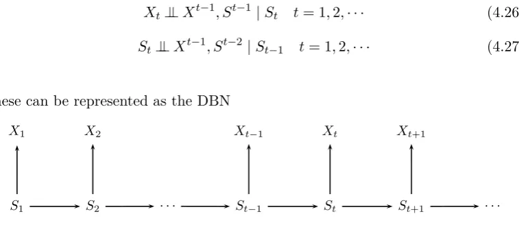
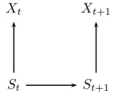
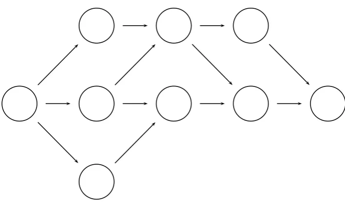
4.1 Dynamic Bayesian network of state-space model . . . 70 4.2 Two-time-slice Bayesian network of state-space model . . . 71 4.3 Example of a ﬂow network . . . 75

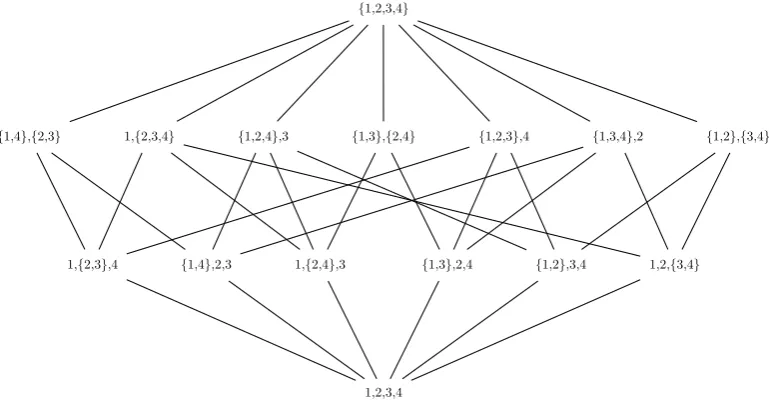
5.1 The Hasse diagram of the lattice of partitions ofS when |S|= 4 . . 89

6.1 The event tree from Example 1 with the numbers representing the number of students in a simulated sample who reached each situation. 112 6.2 Sub-tree of the event tree of possible grades for the MORSE degree

course at the University of Warwick. Each ﬂoret of two edges de-scribes whether a student’s marks are available for a particular mod-ule (denoted by the edge labelledA for the ﬁrst module) or whether they are missing (N A). If they are available, then they are counted as grade 1 if are 70% or higher, grade 2 if they are between 50% and 69% inclusive, and grade 3 if they are below 50%. Some illustrative count data are shown on corresponding nodes. . . 113 6.3 Plots of probabilities that each pair of situations are in the same

stage for diﬀerent values of t, for the case when k = 0.9, ρ = 0.9,

q = 0.2 with P(C1 ={v1,v2,_{v3, . . . , v6},_{v7, . . . , v10}}) = 1, using the values in Table 6.2 . . . 114 6.4 Plots of probabilities that each pair of situations are in the same stage

for diﬀerent values oft, for the case whenk= 0.5,ρ= 0.25,q = 0.05

(9)

6.5 Plots of probabilities that each pair of situations are in the same stage for diﬀerent values oft, for the case whenk= 0.5,ρ= 0.25,q = 0.05

withP(C1 ={v1,v2,_{v3, . . . , v6},_{v7, . . . , v10}}) = 1, and situations

(10)

Acknowledgments

This thesis was typeset with La_{TEX, with the help of the}warwickthesispackage put together by someone from the Physics department. In fact, I owe many people who I have never met and likely never will for the smorgasbord of open-source and Free (not just in price) software that I used during my PhD research, including the TEX stable. I transitioned from Microsoft Windows to the GNU/Linux operating system, currently in the form of the openSUSE distribution, and am eternally grateful for the opportunity to do so. To choose only a few other programs from the multitude that I don’t have the time or memory to acknowledge here explicitly, I would like to thank the many authors and other contributors to GNU Emacs, gcc/g++, KDE and, most of all, the statistical programming language and interpreter R, in which I carried out the analyses of Chapter 6.

Turning to the people who have had a more direct role in helping to bring this thesis to fruition, it is only right that I first thank my supervisor, Professor Jim Q. Smith. He was and is an inspiring and thoughtful mentor who has massively influenced my statistical thinking and even my general approach to life through his effervescent enthusiasm and all-too-rare critical thinking. Thank you for putting up with my quirks so patiently.

(11)

why I appreciate all of them. I have made friends for life, and that is a precious gift that I won’t take for granted.

(12)

Declarations

I hereby declare that this thesis is based on my own research, except when stated otherwise. This thesis has not been submitted for a degree at another university.

Some of this work has been published, accepted for publication or submitted for publication as follows.

The material in Chapter 3, except for the part concerning the weighted MAX-SAT formulation, and some of Chapter 6, has been accepted for publication in the

Journal of Multivariate Analysisunder the title “Bayesian MAP Selection of Chain Event Graphs”. The paper was co-authored with Jim Q. Smith but all the work is mine. Some of the material was also published as [Thwaites et al., 2009]. These papers are also available as CRiSM Working Papers 09-06 and 09-07 respectively.

The material in Chapter 4 is derived from a co-authored invited paper with Jim Q. Smith for the Journal of Forecasting under the title of “Distributional Kalman ﬁlters for Bayesian forecasting and closed form recurrences”. That paper was written with Jim Q. Smith but the text in Chapter 4 is entirely my own work. It is available as CRiSM Working Paper 10-13.

(13)

Abstract

Graphical models provide a very promising avenue for making sense of large, complex datasets. The most popular graphical models in use at the moment are Bayesian networks (BNs). This thesis shows, however, they are not always ideal fac-torisations of a system. Instead, I advocate for the use of a relatively new graphical model, the chain event graph (CEG), that is based on event trees.

Event trees directly represent graphically the event space of a system. Chain event graphs reduce their potentially huge dimensionality by taking into account identical probability distributions on some of the event tree’s subtrees, with the added beneﬁts of showing the conditional independence relationships of the system — one of the advantages of the Bayesian network representation that event trees lack — and implementation of causal hypotheses that is just as easy, and arguably more natural, than is the case with Bayesian networks, with a larger domain of implementation using purely graphical means.

The trade-off for this greater expressive power, however, is that model spec-ification and selection are much more difficult to undertake with the larger set of possible models for a given set of variables. My thesis is the first exposition of how to learn CEGs. I demonstrate that not only is conjugate (and hence quick) learning of CEGs possible, but I characterise priors that imply conjugate updating based on very reasonable assumptions that also have direct Bayesian network analogues. By re-casting CEGs as partition models, I show how established partition learning algorithms can be adapted for the task of learning CEGs.

(14)

Chapter 1

Introduction

Very large datasets are becoming ever more common, with the ability to make sense of them becoming a major problem [Lohr, 2009]. If one uses overly simplistic models to analyse them, there is a risk of jumping to incorrect conclusions; if the models are too complex, they can at best take a very long time to compute, and at worst be opaque black boxes that have no explanatory power, cannot be quality-assured and are extremely sensitive in unpredictable ways to hyper-parameter inputs.

Graphical models provide an attractive middle way [Lauritzen, 1996]. Be-cause of their pictorial form, graphs are excellent tools for eliciting expert opinion about a system and are transparent and communicable; because of their highly structured modular form, they can easily be operationalised for computation.

(15)

cannot fully or eﬃciently represent certain common scenarios [Smith et al., 1993]. These include situations where the state space of a variable is known to depend on other variables, or where the conditional independence between variables is itself de-pendent on the values of other variables, calledcontext-specific independence

in the literature [Boutilier et al., 1996]. In order to overcome such deficiencies, enhancements have been proposed to the canonical Bayesian network. Poole and Zhang [2003], for example, definecontextual belief networks. These, however, don’t represent the context-specific independence relationships graphically, thus un-dermining the rationale for using a graphical model in the first place. Boutilier et al. [1996], meanwhile, keep the BN in place but additionally uses trees to describe the structures of the conditional probability distributions.

(16)

combin-ing the subtrees that describe identical subprocesses so that the CEG derived from a particular ET has a simpler topology while in turn expressing more conditional independence statements than is possible through an ET.

Consider the following example, which exempliﬁes the types of hypotheses I plan to search over in my model selection.

Example 1. Successful students on a one year course study components A andB,

but not everyone will study the components in the same order: each student will

be allocated to study either module A or B for the ﬁrst 6 months and then the

other component for the ﬁnal 6 months. After the ﬁrst 6 months each student will be

examined on their allocated module and be awarded a distinction (denoted withD), a

pass (P) or a fail (F), with an automatic opportunity to resit the module in the latter

case. If they resit then they can pass and be allowed to proceed to the other component

of their course, or fail again and be permanently withdrawn from the programme.

Students who have succeeded in proceeding to the second module can again either

fail, pass or be awarded a distinction. On this second round, however, there is no

possibility of resitting if the component is failed. With an obvious extension of the

labelling, this system can be depicted by the event tree given in Figure 1.1.

To specify a full probability distribution for this model it is suﬃcient to only specify the distributions associated with the unfolding of each situation a student might reach. However, in many applications such as this one it is often natural to hypothesise a model where the distribution associated with the unfolding from one situation is assumed identical to another. Situations that are thus hypothesised to have the same transition probabilities to their children are said to be in the same

stage. Thus in Example 1 suppose that as well as subscribing to the ET of Figure 1.1 one would want to consider the plausibility of the following three hypotheses:

(17)

[image:17.595.195.448.102.589.2]

(18)

student passed the ﬁrst module the ﬁrst time or after a resit.

2. The componentsA and B are equally hard.

3. The distribution of marks for the second component is unaﬀected by whether students passed or got a distinction for the ﬁrst component.

Each of these hypotheses can be identiﬁed with a partitioning of the non-leaf nodes (situations). In Figure 1.1 the set of situations is

S ={V0, A, B, P1,A, P1,B, D1,A, D1,B, F1,A, F1,B, PR,A, PR,B}.

The partitionC ofS that encodes the above three hypotheses consists of the stages

u1 = {A, B}, u2 = {F1,A, F1,B}, and u3 = {P1,A, P1,B, PR,A, PR,B, D1,A, D1,B}

to-gether with the singletonu0={V0}. Thus the second stageu2, for example, implies

that the probabilities on the edges (F1,B, FR,B) and (F1,A, FR,A) are equal, as are

the probabilities on(F1,B, PR,B)and (F1,A, PR,A). Clearly the joint probability

dis-tribution of the model – whose atoms are the root to leaf paths of the tree – is determined by the conditional probabilities associated with the stages. A CEG is the graph that is constructed to encode a model that can be speciﬁed through an event tree combined with a partitioning of its situations into stages.

(19)

common Bayesian model selection method, advocated by, for example, Bernardo and Smith [1994], Denison et al. [2002], Heckerman [1999] and Castelo [2002], the latter two speciﬁcally for models that are Bayesian networks. Because the range of possible CEG models foranysystem exceeds the set of possible BN models, however, and encode information diﬀerently from them, the algorithms for searching for MAP BNs must be adapted accordingly. In Section 6.1.1 I show how to learn a CEG from the tree in Example 1 using simulated data and the algorithm developed in Section 3.3.

My aim throughout this thesis is to ensure all calculations, at least with com-plete sampling, are exact, i.e. there is no need for approximate numerical techniques such as MCMC. While MCMC has vastly widened the vista of possible Bayesian analyses, it can sometimes be used as a crutch when a faster, wholly adequate exact analysis would be possible with a slight adjustment of the model. When it comes to very large datasets with a commensurately very large set of possible models, conjugate analyses can vastly speed up searches across the model space. MCMC is extremely useful for estimating parameters of models once the most appropriate choice of model has been identiﬁed, if necessary.

In the second half of the thesis I develop a class of dynamic multivariate graphical models over ﬁnite discrete state spaces based on CEGs for the purposes of prediction, where at each time point the relevant cohort of units data is represented by a diﬀerent CEG. Highly multivariate discrete processes are quite common but to my knowledge have so far not been systematically studied with graphical models. These processes in the most general case tend to have the following characteristics:

(20)

the state spaces of each stage of development, and so on, but the range of possibilities remains ﬁxed.

2. There are various symmetry hypotheses for a given population of units con-cerning which situations in the histories have the same distributions over their immediate developments.

3. The units arrive in discrete time cohorts, assumed here for simplicity to be equally spaced apart. The symmetries in the system are allowed to change from one time point to the next to reﬂect a changing environment.

4. The system may, at various times, be subject to local interventions, i.e. one of its variables is manipulated exogenously. The model then admits a “causal” extension which provides predictions of the process when subject to such a control.

I am particularly interested in making good one-step ahead predictions for such a system. I consider making good (probabilistic) predictions (orforecasts) to be the central goal of statistical analysis, as argued by de Finetti [1974] and Dawid [1984]. This approach will also provide, as a beneﬁcial side-eﬀect, the probabilities of the symmetry hypotheses through time, which can be used as an explanatory tool.

One example of a system that ﬁts the criteria above is a programme of study provided by an educational establishment which monitors students’ marks over time. The general points above then translate into the following speciﬁc issues:

(21)

v1

v2

A

v4

1

v8

v5

2

v9

v6

3

v10

v3 N A

[image:21.595.231.412.104.351.2]

v7

Figure 1.2: Event tree for marks for two modules in a course. Marks are discretized into 3 grades, andAandN Aindicate whether the mark is recorded or missing. The 10 situations are labelled and the 16 leaf nodes are unlabelled.

2. A student’s performance on a previous module could inﬂuence the marks on a later one.

3. New students come in yearly cohorts. Because of any number of possible changes in any number of unobserved confounding factors the similarities in outcomes between diﬀerent course histories could change for each cohort.

4. The administrators will be interested in predicting the eﬀect on the mark dis-tribution by changing the program in some way, such as changing the syllabus or lecturer for a module, changing the prerequisites for a modules, or removing a module entirely.

(22)

The event tree can represent any discrete event space and naturally codiﬁes a chronological order (or partial order) in its topology, and so I base my own dynamic graphical model on it. However, it is not suﬃcient for addressing the rest of our requirements by itself, particularly because it does not codify the symmetries in the system that I am interested in modelling. CEGs do, though, and so the model class developed here is based on them but extended into a more general dynamic scenario where probabilities and symmetries are allowed to change with time.

I describe the dynamics of this type of tree-structured process by a state space model incorporating a switching mechanism to neighbouring models at every time point. The earliest example of this general class, to the best of my knowledge, was studied for univariate Gaussian series [Harrison and Stevens, 1976; West and Harrison, 1997] and called Multi-process Models Class II. Frühwirth-Schnatter [2006] reviews switching models for non-Gaussian state spaces, but none of these have closed posterior forms. Here, I use a type of multi-process model which allows dynamic shifting from one symmetry partition to neighbouring ones whilst retaining conjugacy.

Various classes of discrete multivariate time series are of course well studied. Possibly the closest classes to the one considered here with associated graphical models are the models used in event history analysis. Event history data relates to when events of interest occur, rather than what events occur at time points of interest. Formally, an event history can be identiﬁed as amarked point process, a set{(Ts, Es) :s= 1, . . . , S} of pairs of timesTs when events Es occurred, where

(23)

event history data and the problem outlined here, it is clear that the two address quite separate concerns. In event history analyses the number of events under consideration is typically small, with the focus of analysis being the timing of events, usually allowed to occur within a continuous time domain. Here, in contrast, I wish to model a class of complex discrete distributions over a discrete time domain. I discuss the connections between the two model classes further in Chapter 7.

In order to take into account possible drifting on the tree parameters through time caused by unobserved background processes, one could follow the standard approach of stating a transition probability P(θt|θt−1, S), where θt represents the

parameters on the tree at timetandS is the underlying model. The most common way to achieve this is to use a conventional state-space formulation. Unfortunately, this approach almost always immediately requires the inference to be undertaken with approximating numerical methods. This is not ideal in this context for several reasons: First, in the process I consider here, conjugacy and modularity are present and it would be a shame to lose these useful properties. Secondly, because of the vastness of the model space of our domain of application it is convenient to be able to have Bayes factors calculable in closed form, because this greatly speeds up computation of model goodness. Thirdly, models in this class are easier to interpret when they retain their modular and conjugate forms.

An alternative approach, which I take here, is to set a transition function

T :P(θt−1 |xt−1, S)7→P(θt|xt−1, S) (1.1)

(24)

several diﬀerent authors to use such transitions. I also show that it has the property of preserving the modular structure of each model in this class and works well against prior misspeciﬁcation.

Interventions on a graphical model are covered by the causal literature (e.g. Pearl [2000b]). Causal analysis on event trees was considered by Shafer [1996] and was deﬁned for static chain event graphs by Thwaites et al. [2010]. I extend this to the dynamic model class presented here. By still retaining conjugacy and modularity when learning model probability parameters, this causal extension of the model class is particularly straightforward, allowing it to be easily used for modelling a controlled environment.

Thesis outline

The remainder of this thesis is thus structured as follows.

In Chapter 2 I review the latest theory concerning graphical models and how to learn them automatically.

In Chapter 3 I review the deﬁnitions of event trees and CEGs. I then develop the theory of how conjugate learning of CEGs is performed, and apply this theory by using the posterior probability of a CEG as its score in a model search algorithm that is derived using an analogous procedure to the model selection of BNs. I characterise the product Dirichlet distribution as a prior distribution for the CEGs’ parameters under particular homogeneity conditions.

In Chapter 4 I review some theory concerning state-space and dynamic graph-ical models that will be relevant in developing the new dynamic graphgraph-ical model based on CEGs.

(25)

predictions with the new model. I then extend the model to allow the implementa-tion of causal analyses.

In Chapter 6 I apply all of the theory and algorithms to a simulated data for testing purposes and then to results from a real educational programme in order to make rich inferences about students’ educational achievement.

(26)

Chapter 2

Graphical models

I begin by describing what I consider graphical models to be and why they are worthy of study and use. I then move on to discussing various statistical issues concerning the most popular contemporary graphical model: the Bayesian Network (BN). I ﬁnish by critiquing the BN and proposing a new graphical model that is more appropriate for many applications based on trees.

2.1 Introduction to graphical models

Statistical models are descriptions of stochastic systems that enable us to understand the relationships between the variables of that system. In the Bayesian paradigm, the statistical model encodes degrees of belief about various hypotheses concern-ing the system as probabilities, and these probabilities are updated in line with probability theory as observations of the system are made.

(27)

aﬀect any analysis adversely. Excessively complex models, however, require the set-ting of more parameters, which leads to greater risk of model mis-speciﬁcation, and also large amounts of computation which can quickly lead to intractability. What is required, as Einstein put it, is “to make the irreducible basic elements as simple and as few as possible without having to surrender the adequate representation of a single datum of experience” [Einstein, 1934]. One way to do so is to make qual-itative judgements about the system, for example about any homogeneities which are believed a priori to exist between seemingly separate variables. This can reduce the dimensionality of the model as well as increase its power. To represent these statements transparently one can use a (network) graph, which characterises the model as a graphical model.

Lauritzen [1996] notes that graphical models have their origin in the early 20th century in the analysis of statistical mechanics by Gibbs [Gibbs, 1902; Borgelt and Kruse, 2002]. Nowadays graphical models are considered to be “statistical mod-els embodying a collection of marginal and conditional independences which may be summarized by means of a graph” [Dawid and Lauritzen, 1993]. This certainly describes Bayesian networks, but I will show how the syntax of a graph can be used to describe other model properties apart from independence relationships.

My overarching aim when using graphical models is well described by Dawid [2002]:

Seek to represent and manipulate as much as possible of the relevant structure and details of the model by purely graphical means, keeping any external information required to a minimum

(28)

I begin by revising basic graph theory terminology that will be used through-out. Further details of these concepts can be found in many introductory graph theory texts, e.g. [West, 2001].

Deﬁnition 2. AgraphG is a pair(V(G), E(G)) whereV(G) is its set of vertices

(or nodes),E(G)is its set of edges. The set of edges can be thought of as a relation

onV(G).

When a graph is drawn, the vertices are displayed as points and the edges as

curves between the appropriate points.

Deﬁnition 3. A directed graph (or digraph) is a graph G where the edges are

ordered pairs of vertices. Thus the edges e1 = (v1, v2) and e2 = (v2, v1) (where

v1, v2∈V(G)) are distinct elements ofE(G).

Edges in a directed graph are drawn as arrows from the ﬁrst vertex to the

second vertex in the ordered pair.

All graphs in this paper are directed graphs, and the following deﬁnitions

assume this.

Deﬁnition 4. In a digraph, the child of the edge e = (v1, v2) ∈ E(G), written

ch(e), is v2. Its parent pa(e) is v1.

By abuse of notation, the children of a vertex v∈ V(G), written ch(v), are

deﬁned as

ch(v) ={v′ :v′ ∈V(G),(v, v′)∈E(G)} (2.1)

andpa(v) is deﬁned similarly.

Deﬁnition 5. A pathλ between two verticesv1, v2∈V(G) is an ordered sequence

of edges λ(v1, v2) = (e1, . . . , en) where e1, . . . , en∈E(G), pa(e1) = v1, ch(en) = v2

(29)

Deﬁnition 6. The length of a path is the number of edges it contains, given in

the above deﬁnition as n. By an abuse of notation, we say v ∈λ (where v∈V) if

the pathλ passes through v.

Deﬁnition 7. A cycleis a path λ(v1, v2) where v1 =v2.

Deﬁnition 8. Anacyclic graph contains no cycles.

Deﬁnition 9. A graph is connected if there exists a path in the graph between

every pair of vertices, where direction of edges here can be changed if necessary.

Deﬁnition 10. A graph is a completegraph if there is an edge between every pair

of nodes.

Deﬁnition 11. Atreeis a connected acyclic graph where one vertex (denoted here

by v0) has no parents and all other vertices have exactly one parent.

Deﬁnition 12. A leaf nodein a tree is a vertex with no children. The set of leaf

nodes of a tree T is denoted here by L(T).

2.2 Introduction to Bayesian networks

The Bayesian network uses a modification of the graph theory concept of separa-tion to represent condisepara-tional independence relasepara-tionships. It can be proven that the separation properties of a Bayesian network graph match up with the conditional independence properties of a statistical model so that such a representation makes sense. I show here how this is done formally, beginning with giving the definition and formal axioms of conditional independence as defined by [Dawid, 1979]. The axioms are also called thesemi-graphoid axioms after Pearl and Paz [1986].

(30)

Deﬁnition 13. Let X, Y, Z be random variables on a probability space (Ω,F, P).

Then X is conditionally independent of Y given Z (under P) if for any

P-measurable set A in the sample space of X, P(X ∈A|Y, Z) can be expressed as a

function ofZ alone.

It is clear that conditional independence is a useful modelling assumption to make if it sensible to do so, because the dimensionality of the model for any random variable can be reduced when conditioning on other variables. A special case of this phenomenon is statistical suﬃciency, as explained by [Dawid, 1979; Dawid and Lauritzen, 1993], when the random variables are parameters of the model; another example of conditional independence is in linear regression where the number of explanatory variables required in the model is deemed to be suﬃcient to model the dependent variable.

Standard independence holds when Z in the above deﬁnition is the empty set.

Now I introduce the semi-graphoid axioms. Let W, X, Y, Z be four disjoint subsets of a setU and let _⊥_⊥ and _|form a ternary relationR⊆U3 of subsets of U, where I write X⊥⊥Y|Z if (X, Y, Z) ∈ R, for example. It is also possible to write

X⊥⊥Y if (X, Y,∅) ∈ R. R then satisﬁes the semi-graphoid axioms if, as given by [Borgelt and Kruse, 2002],

Symmetry (X⊥⊥Y |Z) =_⇒ (Y ⊥⊥X |Z)

Decomposition ((W ∪X)⊥⊥Y |Z) =_⇒ (W ⊥⊥Y |Z) and (X⊥⊥Y |Z)

Weak union ((W ∪X)⊥⊥Y |Z) =⇒ (X⊥⊥Y |Z∪W)

Construction (X⊥⊥Y |(Z∪W))and (W ⊥⊥Y |Z) =_⇒ ((W ∪X)⊥⊥Y |Z)

(31)

and therefore we can writeX⊥⊥Y |Z to represent the statement that X is condi-tionally independent of Y given Z.

I now show how a Bayesian network can be used to graphically represent all of the conditional independence statements of a model.

Deﬁnition 14. A Bayesian network for the model with set of random variables

X ={X1, . . . , Xn} on a probability space (Ω,F, P) is a directed acyclic graph G=

(V, E) where

1. each node Vi ∈V corresponds to exactly one variable Xi∈X, and

2. ifP(X) can be written as ∏n_i₌₁P(Xi |Qi), whereQi ⊆ {X1, . . . , Xi−1} (with

the exception of Q1 = ∅), then pa(Vi) = V(Qi), where V(Qi) are the nodes

corresponding to the random variables inQi.

From here on in, I refer to the vertices representing random variables or sets or collections of random variables by the random variables themselves, except in cases where there might be possible confusion.

Note that a complete Bayesian network can always be drawn for a model with a ﬁnite number of random variables, asP(X1, . . . , Xn) =

∏n

i=1P(Xi|X1, . . . , Xi−1)

is always true. Note therefore that there may also be more than one possible Bayesian network representation of a model; in particular, any complete directed acyclic graph withV =V(X)is always a valid Bayesian network. Adding edges to a valid BN always creates another valid BN, as long as the resulting graph remains directed and acyclic.

It is clear the Bayesian network representation of a model explicitly encodes some conditional independence statements of the model. Speciﬁcally, it can be immediately read from the graph that

(32)

fori= 2, . . . , n purely from its topology. However, more conditional independence statements can be inferred from the graph using a property of the graph that also satisfies the semi-graphoid axioms. This property isd-separation, first defined by Verma and Pearl [1988] and subsequently re-defined by Lauritzen [1996] in a more useful and operational way, where for three disjoint subsets A, B, S ⊂V, S is said to d-separateAand BifSblocks all paths between all vertices in Aand all vertices inB on a transformed version of the original BN. The transformation is as follows:

1. Delete all vertices from the BN that are neither part ofA,B orS, nor have a path from themselves to another vertex inA,B orS. Delete all edges which had one of the deleted vertices at one of their ends. This is theancestral

graph of the BN.

2. For every pair of nodes that have a common child that are not connected create an edge between them. This is the moralised graph (because “unmarried” parent nodes are made to “marry”).

3. Ignore the directions of arrows on edges for determining whether paths are blocked. This is theskeletongraph.

Then it can be proven that for any BN set up as above,

S d-separatesA from B=⇒A⊥⊥B |S (2.3)

(33)

2.3 Learning Bayesian networks

In many scenarios, the modeller might not have complete certainty over the condi-tional independence relationships which hold between the variables of the system under consideration, or equivalently the Bayesian network which best represents the model. In this case, the Bayesian approach is to consider the structure itself as a random variable with a probability distribution of its form set a priori, and then updated using Bayes’ theorem in the light of new data. This procedure has been de-scribed aslearningthe Bayesian network by the artiﬁcial intelligence community, e.g. in [Heckerman, 1999] and can be considered as another form of model selection. However, the procedure is in practice rarely so simple. The major obstacle in carrying it out is that the size of the set of possible Bayesian networks grows in size super-exponentially with respect to the size of the set of random variables [Cooper and Herskovits, 1992]. This means that setting a proper subjective prior distribution over the set of possible Bayesian networks for any practical situation is generally intractably diﬃcult, as is setting the parameter priors and likelihoods for each possible BN.

There are some approaches advocated in the literature, however, that seek to minimise this diﬃculty by utilising some reasonable simplifying assumptions. I discuss the assumptions which relate to discrete variables in particular which is my focus in this thesis.

The initial set of assumptions deals with the probability model for the data implied by each Bayesian network. LetB be the random variable representing the Bayesian network which holds. Then

P(X |θB, B) = n ∏

i=1

(34)

where θB = {θB1, . . . , θBn} is the set of parameter vectors θBi for each

distribu-tion P(Xi | Qi, θBi, B). Then the prior probability distribution of θB|B is set by

assumingparameter independence[Spiegelhalter and Lauritzen, 1990], so that

P(θB|B) = n ∏

i=1

qi

∏

j=1

P(θBij |B) (2.5)

where θBij is the parameter vector of the probabilities P(Xi | Qi = qj, B) and qi

is the number of possible values of Qi. Note that I am assuming, in line with my

relevance assumptions, that the value of θBij does not rely on the parts of B not

related to Xi and its parents, a property called likelihood modularity. If θBij

is distributed as Dir(αBij), then the updating ofP(θBij |B,X) is conjugate:

θBij |B,X ∼Dir(αBij+Nij) (2.6)

whereNij represents the vector of counts Nijk when Qi =qj and Xi =xik, where

kindexes the possible values of Xi.

While parameter independence simpliﬁes the setting and updating of P(θ | B) for each possible BNB, it still requires the setting of each P(θBij|B) for each

B, and still does not address the setting ofP(B).

In order to simplify the setting ofP(θBi |B)— the priors for the parameters

of variable Xi in a BN B — for all variables Xi for each possible BN B, one can

make the assumption of prior modularity. This states that if two Bayesian networks B1 and B2 have identical parent variables Qi for some variable Xi, then

P(θBi | B1) = P(θBi | B2), i.e. the prior on the parameters that determine the

distribution ofXi are equal for both BNs. The subscriptBwill therefore be dropped

(35)

Under the assumptions of prior and likelihood modularities, it is the case (as shown in [Heckerman and Geiger, 1995]) that in order to set parameter priors for each possible BN it is suﬃcient to set parameter priors only for the complete Bayesian networks. Parameter priors for incomplete networks are then derived from equivalent local structures in the corresponding complete network.

This can still be intractable, and so there is one more level of simpliﬁcation possible. Assume that under any B the parameter vectors θij are mutually

inde-pendent of one another for any Xi for any values of its parents Qi =qj as above,

and that for any two Markov equivalent BNs B1, B2 (i.e. those which encode the

same sets of conditional independence relations onX, as can be determined using the methods of [Verma and Pearl, 1990] or [Chickering, 1995]) it is assumed that

P(X |B1) =P(X |B2) (called hypothesis equivalence by [Heckerman et al., 1995]). Geiger and Heckerman [1997] showed that in this case that allθij must have

a Dirichlet distribution. Therefore to specify the parameter priors for any network

B one needs only to specify the hyperparameters of the Dirichlet distribution of the joint distribution ofX on a complete network.

The setting ofP(B)is comparatively simple. Apart from the obvious choices of a uniform prior over all possibleB or a subset of all possible B, another possible qualitative characterisation is to consider the probability for the inclusion of each edge in a BN with a ﬁxed order of variables [Buntine, 1991], and further still if the edges are considered exchangeable, i.e. all of the edges have a probability p of existing, then only one probability assessment — that ofp — is needed.

With the parameters set as above and assuming Dirichlet priors,P(X |B)

(36)

Heckerman et al. [1995]:

P(X |B) =

n ∏

i=1 |qi|

∏

j=1



 Γ(αij.)

Γ(αij.+xij.)

|xi|

∏

k=1

Γ(αijk+xijk)

Γ(αijk) 

 (2.7)

where|xi|are the number of possible values ofXi,xij. = ∑

kxijk,xijkis the number

of times Xi =xik when Qi =qj, and αij. = ∑

kαijk. P(B |X) can then be easily

calculated from Bayes’ theorem for eachB ifP(B) is a ﬁxed quantity a priori. However, when there are a large number of possible BNs B, this might not be practical. To predict new dataX∗ from the system after having observedX, it is necessary to calculate

P(X∗ |X) = ∑

B∈B

P(X∗|B)P(B |X). (2.8)

This is calledmodel averaging [Hoeting et al., 1999]. For a large set of possible BNs B, it would be impractical to calculate P(X∗ | B) and P(B | X) for each

B. There are a number of approximations to the full solution which could still give good predictions while reducing the computational eﬀort required [Hoeting et al., 1999].

If the aim is to provide a good “explanatory” network for the system, then trying to find the most probable BN (MAP, or Maximum A Posteriori BN) can be done more efficiently, if not necessarily optimally, than just calculatingP(B|X)for every possibleB, bysearchingthe model space. There have been many strategies suggested for this search, including greedy search, greedy search with restarts, best-first search, and Monte Carlo methods, all discussed by Heckerman [1999], and more recently weighted MAX-SAT solving [Cussens, 2008].

(37)

can be calculated as the product of purelylocal properties of the network, where local here relates to individual nodes and their parents. This means that if two BNs diﬀer only in one parent set Qi of some variable Xi, the diﬀerence in scores

will result only from that local difference. This allows for efficient local search algorithmsfor searching the model space. A simple local greedy search starts with one possible BN, then calculates the score for a BN which differs only in having an edge reversed, an edge added or an edge deleted (subject to the resulting network being acyclic) by only re-calculating the relevant local score, and chooses the BN which has the higher posterior probability. Because only the local differences in the graphs have to be taken into account, the search proceeds more quickly.

The search algorithms to ﬁnd the MAP BN can also be used to ﬁnd more than one high-scoring network so thatP(X∗|X) can be approximated as

P(X∗|X)≈ ∑

B∈B˜

P(X∗ |B)P(B|X) (2.9)

whereB˜ is the set of highest-scoring networks found during the model search, where the size of the set can be chosen as high as desired.

2.4 Causal Bayesian networks

Eﬀorts have been made to use Bayesian networks not only to incorporate beliefs about the conditional independence relations between the variables in a system, but also causal relations between them, most prominently by Pearl [Pearl, 2000b]. I brieﬂy review how this is done and how it has led to work on learning these causal relations.

(38)

network of a system, there can be a conscious or unconscious desire to somehow rep-resent certain “causal” relations between the variables. One way to describe these causal hypotheses is to consider how the system changes under external interven-tion. If a variableA is a cause of another B, then directly changing A will change the probability distribution of B. Pearl [Pearl, 2000b] represents the probability distribution of B after intervening in the value of A as P(B | do(A)), in order to distinguish this distribution from the one ofB after merely observingA,P(B|A). There is no reason why in general P(B | do(A)) should be related to P(B | A), but in many cases there is a presumed relationship that can be incorporated into a model.

A causal Bayesian network (CBN) [Pearl, 1995] sets strict constraints on this relationship. A CBN is a BN that, as well as describing the conditional independence statements that are satisﬁed by the joint probability distribution over the model’s variables, asserts certain beliefs about the probability distribution over the variables resulting from an exogenous manipulation of any subset of them. The exact nature of these beliefs is described in the following deﬁnition.

Deﬁnition 15. A causal Bayesian network is a Bayesian network that

addition-ally holds the following properties when some subset of the variables XI ⊆ X is

intervened upon to take the vector of values xI:

1. The probability distribution of each XI ∈ XI becomes degenerate, so that

P(XI =xI) = 1 when xI is the relevant value from xI, and 0 otherwise

2. The probability distributions of all other variables Xi ∈/ XI conditional on

their parent variables Qi stay unchanged.

(39)

factorisa-tion of the joint probability distribufactorisa-tion described by a BN. Note that now BNs which were describing identical conditional independence statements have diﬀerent replacement probability distributions under identical interventions.

There have been attempts to learn CBNs from data, e.g. by Heckerman [1995], Cooper and Yoo [1999], and Spirtes et al. [2001]. The approach advocated by the ﬁrst two papers cited works by either considering, in addition to the random variables under investigation, whether those variables were merely observed or ac-tively manipulated for each data point, which essentially expands the event space. This is equivalent to re-drawing the CBN as a BN with additional nodes indicating whether manipulation or mere observation led to other nodes’ values, as advocated by Dawid [2002] and called an augmented DAG by him. This BN can then be learnt in the same way as discussed earlier.

(40)

2.5 Disadvantages of Bayesian network representations

Despite their obvious strengths in allowing for the reduction in the dimensionality of models’ joint probability distributions and in providing a transparent framework for causal inference as described above, BNs are not optimal graphical models in all situations. The biggest problems with their use occur under two scenarios, which are not necessarily mutually exclusive:

1. when the model event space is not a simple product space, i.e. the state spaces of some of the random variables in the system are radically diﬀerent — or even non-existent — depending on the values of other system variables; and

2. when conditional independence statements are true only under certain values of other variables.

Neither of these scenarios can be discerned directly from the BN. Consider the situation in Figure 1.2. The event space is clearly asymmetric because if the first module’s marks are unavailable then they have no grade. Additionally, it might be the case, for example, that students who get grades 2 or 3 in the first module perform in an identical way on the second module, but student who perform the best in the first module by getting the highest grade perform completely differently. These features will not be exhibited by the structure on a BN unless special care is taken.

(41)

kept the BN in place but additionally used trees to describe the probability distribu-tions of each variable, and then proceeded to re-arrange the BNs using these trees, including having multiple nodes for a single random variable in order to represent some of the context-speciﬁc independences in a BN format. Jaeger [2004] deﬁned

probability decision graphs(PDGs) that can represent certain context-speciﬁc independences, but PDGs cannot represent some conditional independence relations that can be represented by BNs; for example, as admitted by Jaeger [2004], the BN with nodesX1, X2, X3, X4 and edges (X1, X2),(X1, X3),(X2, X4),(X3, X4) cannot

be represented as a PDG. More recently, [Poole and Zhang, 2003] deﬁned contex-tual belief networks, but these are basically BNs with the extra contextual information not represented graphically.

One final approach is that of Bayesian multinets [Geiger and Heckerman, 1996], where context-specific independence is termedasymmetric independence. Bayesian multinets are essentially collections of different BNs over the same set of random variables, one BN drawn for each collection of values of one of the variables (called thehypothesis variable) that makes the BN of the system different from all the others. While this solves the problem of representing context-specific inde-pendence graphically and hence explicitly, there is still a lot of redundancy in the representation due to needing to draw a BN for each of the variable values of each hypothesis. This problem only gets worse if more than one hypothesis variable is proposed. There is also no acknowledgement of how to deal with sparse conditional probability tables efficiently.

(42)

(43)

Chapter 3

Learning chain event graphs

Finding that the BN is not always the optimal graphical model for modelling certain systems and processes, this chapter suggests the advantages of using a graphical model based on event trees — the chain event graph — and develops a totally new mechanism to learn CEGs from data, from characterised priors to intelligent learning algorithms.

3.1 Prerequisites

3.1.1 Event Trees

(44)

anomaly. Finally, event trees have a perfect match between their topology and the sample spaceΩof the Kolmogorov probability triple (Ω,F, P) of a probability model, ensuring that no aspect of the model is ignored in the graphical represen-tation, while Bayesian networks focus on random variables which are real-valued functions of events.

I start by deﬁning event trees formally.

Let T = (V(T), E(T)) be a directed tree where V(T) is its node set and

E(T) its edge set.

Deﬁnition 16. The set of situations of T, S(T), is the set of non-leaf nodes

{v:v∈V(T)\L(T)}, where L(T) is the set of leaf nodes of T.

Let_Xbe the set of root-to-leaf paths of T, so that _X={λ(v0, v) :v∈L(T)}

(recall that v0 is the root node). _X represents the event space of the model, with every root-to-leaf path an atom of the event space.

In an event tree, each situationv∈S(T) has an associated random variable

X(v) deﬁned conditional on having reachedv. The state space ofX(v) is denoted as_X(v), represented in the tree by ch(v).

Deﬁnition 17. The distribution of X(v) is determined by the primitive

proba-bilities{π(v′|v) =P(X(v) =v′) :v′ ∈X(v)}.

The probability of an eventλ∈Xcan therefore be calculated by multiplying the primitive probabilities along the path. Conversely, primitive probabilities can be inferred from the probabilities for the events inX.

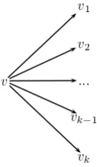
Deﬁnition 18. The floret of v∈S(T) is

(45)

[image:45.595.286.355.106.224.2]

Figure 3.1: Floret ofv. This subtree represents both the random variableX(v)and its state space_X(v).

Figure 3.2: Simple event tree. The non-zero-probability events in the joint prob-ability distribution of two Bernoulli random variables, A and B, with A observed beforeB, can be represented by this tree. Here, all four joint states are possible and hence there are four root-to-leaf paths through the nodes.

where V(F(v)) = {v} ∪ {v′ ∈V(T) : (v, v′) ∈ E(T)} and E(F(v)) = {e ∈ E(T) :

e= (v, v′)}.

The ﬂoret of a vertexvis thus a sub-tree consisting ofv, its children, and the edges connecting v and its children, as shown in Figure 3.1. The ﬂoret represents the situationv, the associated random variableX(v) and its sample spaceX(v).

Example 19. Figure 3.2 shows a tree for two Bernoulli random variables,AandB,

withAoccurring beforeB. In an education setting A could be the indicator variable

of a student passing one module, and B the indicator variable for a subsequent

[image:45.595.257.384.285.375.2]

(46)

Here we have random variablesX(v0) =A,X(v1) =B|(A= 0)andX(v2) =

B|(A= 1), and primitive probabilitiesπ(v1|v0) =p(A= 0),π(v3|v1) =p(B = 0|A=

0) and so on for every other edge. Path probabilities can be found by multiplying

primitive probabilities along a path, e.g. p(A = 0, B = 0) = p(A = 0)p(B = 0|A =

0) =π(v1|v0)π(v3|v1) as (v0, v1) and (v1, v3) are on the path between v0 and v3.

3.1.2 Chain Event Graphs

Starting with an event tree T, we extend the deﬁnition with three new concepts to form the CEG — stages, edge colours and positions – similarly to the approach of [Smith and Anderson, 2008] and [Thwaites et al., 2010].

One of the redundancies that can be eliminated from an ET is that of two situations, v and v′ say, which have identical associated edge probabilities despite being defined by different conditioning paths. We say these two situations are in (or at) the samestage. This concept is formally defined below.

Deﬁnition 20. Two situations v, v′ ∈S(T) are in the same stage u if and only if

X(v) andX(v′) have the same distribution under a bijection

ψu(v, v′) :X(v)→X(v′) (3.1)

Deﬁnition 20 means that every pair of situations in a stage have a bijection between their sample spaces that identiﬁes which pairs of outcomes have equivalent probabilities.

The set of stages of an event treeT (also called itsstaging) is writtenJ(T). This set partitions the set of situationsS(T), due to the associated set of bijections

{ψu(v, v′) :v, v′∈u, u∈J(T)} forming an equivalence relation onS(T).

(47)

only if v, v′ ∈ u ∈ J(T) and ψu(v, v′)(v∗) = v′∗, i.e. v∗ and v′∗ are considered to

have equal probabilities of being reached fromv and v′ respectively.

The edge colours make it clear, when drawn, which edges represent the same primitive probabilities and hence which situations are in the same stage. An al-ternative approach is to indicate which situations are in the same stage is to draw undirected edges between them, as in [Smith and Anderson, 2008; Thwaites et al., 2010].

Sometimes two situations have even more in common than the distribution over their respective variables: the entire subtrees with the two situations as roots share the same distribution over their paths. These two situations are said to be in the sameposition. I deﬁne this concept formally.

Deﬁnition 22. Two situationsv, v′ ∈S(T)are in the samepositionwif and only

if there exists a bijection

ϕw(v, v′) : Λ(v, T)→Λ(v′, T)

where Λ(v, T) is the set of paths in T from v to a leaf node of T, such that for

every pathλ(v)∈Λ(v, T), the ordered sequence of colours inλ(v)equals the ordered

sequence of colours inλ(v′) :=ϕw(v, T)(λ(v))∈Λ(v′, T)

I denote the set of positions asK(T). It is clear thatJ(T) is a partition of

K(T), as situations in the same position are in the same stage. K(T) is therefore a ﬁner partition ofS(T) thanJ(T).

Now the CEG can ﬁnally be constructed by taking the staged treeU(T) of an event tree and merging situations that are in the same position.

Deﬁnition 23. The chain event graph (CEG) C(T) of an event tree T is the

(48)

• V(C) = K(T)∪w_∞, so that each non-leaf node in the CEG represents one

position and w_∞ represents the set of leaf nodes.

• Each edge in E(C) exists for one of the following two reasons.

– Forw, w′ ∈V(C)\w_∞, there is an edge(w, w′)∈E(C)if and only if there

exist situations v, v′ ∈S(T) such that v∈w, v′ ∈w′ and(v, v′)∈E(T).

– For w ∈ V(C)\w_∞, there is an edge (w, w_∞) ∈ E(C) if and only if

there exist situations v ∈ S(T) and v′ ∈ L(T) such that v ∈ w and

(v, v′)∈E(T).

• The edge (w, w′)∈E(C) has the same colour as (v, v′) ∈E(T) where v ∈w,

v′ ∈w′.

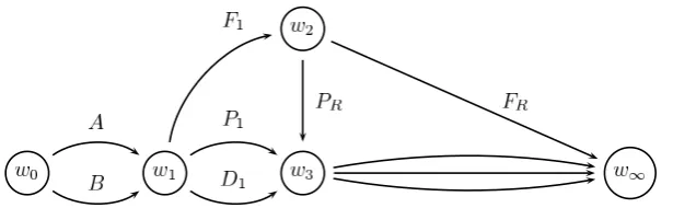
An example of a CEG that could be constructed from the event tree in Figure 1.1 is shown in Figure 3.3. It can immediately be seen that the CEG is a more compact representation of the probability distribution over the system than the event tree, but without discarding any information reflected by the tree. The non-leaf nodes in Figure 3.3 are positions representing the three hypotheses described in Chapter 1. For example,w1 is the position reached after knowing what the first module is; if modules A and B are equally hard then the mark distributions are equivalent whetherA or B is taken first, and hence the subtrees with A and B as root nodes will have identical distributions. The other positions can be identified with the hypotheses of Example 1 similarly.

(49)

[image:49.595.169.477.106.201.2]

Figure 3.3: The CEG that reﬂects the three hypotheses of Example 1

by a CEG through stages and positions as is shown in [Smith and Anderson, 2008] and [Thwaites, 2008]. This is because the CEG works on the level of the event space of the probability model while the BN considers only random variables.

3.1.3 Causal trees and CEGs

There is another aspect to event trees (and hence CEGs) that make their use in modelling extremely appealing: their powerful expressiveness in describing causal hypotheses and learning about the effect of external interventions in the system from observational data. Due to reflecting the event space more finely, the range and realism of the possible causal analyses is better than for a Bayesian network of the same system. The intuitiveness of using trees for modelling causal hypotheses was argued forcefully by [Shafer, 1996].

(50)

through manipulation of the graphical structure itself, because the edges of a BN do not represent parts of the event space but rather the conditional independence structure of the system.

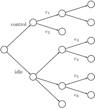
For example, consider the event tree in Figure 3.4 (inspired by an example in [Smith, 2010]) which shows the two possible developments of a process conditional on whether it is left undisturbed (“idle”) or controlled.

control

e1

e2

idle

e3

e4

e5

[image:50.595.227.413.242.455.2]

e6

Figure 3.4: Event tree for idle and manipulated versions of the same process

In Figure 3.4, the probabilities ofe1, e2 might be considered equal to e3, e4

respectively, i.e. the associated variables become independent of whether they are in the controlled or idle system, bute5, e6 might still be considered to be independent.

This cannot be considered graphically with a BN.

In a CEG, the edges will either be coloured the same or merged, making explicit the model assumptions involved and in the latter case doing so eﬃciently. The range of manipulations possible on a CEG is explored further in [Thwaites et al., 2010].

(51)

dynamic version of the CEG where the same edge is considered exogenously to the structure to be equivalent in both the idle and the manipulated versions of the system, and in Section 6.2.2 I demonstrate its use with a real dataset.

3.2 Conjugate learning of CEGs

It turns out that one convenient property of CEGs is that conjugate updating of the model parameters is possible in a closely analogous fashion to that on a BN as described in Section 2.3. Conjugacy is a crucial part of the model selection algorithm that will be described in Section 3.3, because it leads to closed form expressions for the posterior probabilities of candidate CEGs, which in turn makes it possible to search the often very large model space quickly to ﬁnd optimal models. The CEG model class will in general be bigger than the BN class for the same random variables, so that a model search will generally take longer but with the beneﬁt that a richer model class is being considered. I demonstrate here how a conjugate analysis on a CEG proceeds.

Let a CEG C have set of stages J(C) = {u1, . . . , uk}, and let each stage ui have ki outgoing edges (labelled e1, . . . , eki) with associated probability vector πi= (πi1, πi2, . . . , πiki)′ (where

∑ki

j=1πij = 1 and πij >0 forj∈ {1, . . . , k}).

Then under complete sampling, the likelihood of the CEG can be decomposed into a product of the likelihood of each probability vector, i.e.

p(x|π, C) =

k ∏

i=1

pi(xi|πi, C) (3.2)

where π = {π1,π2, . . . ,πk}, and x = {x1, . . . ,xk} is the complete sample data

such that eachxi = (xi1, . . . , xikn)′ is the vector of the sample data of the edges (or

(52)

stageui.

With independence between the units conditional on π (i.e. the units are exchangeable)

pi(xi|πi, C) = ki

∏

j=1 πx

(j) i

ij (3.3)

wherex(_ij) is the number of units which take thejth edge.

Thus, just as for the analogous situation with BNs, the likelihood of a ran-dom sample also separates over components of π. With BNs, a common mod-elling assumption is of local and global independence of the probability parameters [Spiegelhalter and Lauritzen, 1990]; the corresponding assumption here is that the parametersπ1,π2,. . .,πk ofπ are all mutually independent a priori. It will then

fol-low, with the separable likelihood, that they will also be independent a posteriori. If the probabilitiesπi are a priori assigned a Dirichlet distribution, Dir(αi),

whereαi = (αi1, αi2, . . . , αiki)′, then for values ofπwhere

∑ki

j=1πij = 1andπij >0

for1≤j≤ki, the density ofπi,qi(πi|C), can be written

qi(πi|C) =

Γ(αi1+. . .+αiki) Γ(αi1). . .Γ(αiki)

ki

∏

j=1 πα_ijij−1

where Γ(z) = ∫₀∞tz−1e−tdt is called the Gamma function. It then follows that

πi|x (=πi|xi) also has a Dirichlet distribution, Dir(α∗i), a posteriori, where α∗i =

(α∗_i₁, . . . , α∗_ik i)