STABILITY ANALYSIS OF A ROTATING FLOW TOWARD A
SHRINKING PERMEABLE SURFACE IN NANOFLUID
Siti Nur Alwani Salleh*, Norfifah Bachok, and Norihan Md Arifin
Department of Mathematics and Institute for Mathematical Research, Universiti Putra Malaysia, 43400 UPM Serdang, Selangor, Malaysia
*Corresponding Author: [email protected]
Received: 28th Oct 2018 Revised: 28th Oct 2018 Accepted 19th Dec 2018
DOI: https://doi.org/10.22452/mjs.sp2019no1.2
ABSTRACT The rotating boundary layer flow over a shrinking permeable surface in nanofluid is numerically studied. The similarity transformation is used to transform the partial differential equations into nonlinear ordinary differential equations. Later, these equations are determined by using bvp4c package in the MATLAB software. The numerical results reveal that there is more than one solution called dual solutions obtained for a certain range of the rotation and suction parameters. A stability analysis is performed to determine which solution is stable by depending on the sign of the eigenvalues. Based on this analysis, the results indicate that the upper branch solution (first solution) is linearly stable, while the lower branch solution (second solution) is linearly unstable.
Keywords: Dual solutions, nanofluid, rotating flow, shrinking sheet, stability analysis.
ABSTRAK Aliran putaran lapisan sempadan terhadap permukaan mengecut yang telap di dalam nanobendalir dikaji. Penjelmaan keserupaan digunakan untuk menjelmakan persamaan perbezaan separa kepada persamaan perbezaan biasa tak linear. Kemudian, persamaan ini diselesaikan dengan menggunakan pakej bvp4c dalam perisian MATLAB. Keputusan menunjukkan bahawa terdapat lebih daripada satu penyelesaian yang disebut penyelesaian dwi diperolehi untuk julat tertentu bagi parameter putaran dan sedutan. Analisis kestabilan dijalankan untuk menentukan penyelesaian mana yang stabil dengan bergantung kepada tanda nilai eigen. Berdasarkan analisis ini, keputusan menunjukkan bahawa penyelesaian cabang atas (penyelesaian pertama) adalah stabil, sementara penyelesaian cabang bawah (penyelesaian kedua) adalah tidak stabil.
INTRODUCTION
Along with the development of technology in this day and age, the usage of nanofluid became one of the hot issues to some
cooling tool will definitely enhance the
manufacturing processes as well as
operating costs. This fluid is formed by dispersing some of the nanoparticles into the base fluid which is water. After the discovery of nanofluid by Choi (1995), Bachok et al. (2010, 2012), Reddy et al. (2013), Das et al. (2014), Rosca and Pop (2014), Naramgari and Sulochana (2016) and Othman et al. (2017) have attempted to focus their research on the boundary layer flow of nanofluid using different effects and surfaces. Recently, the nanofluid problem with the presence of rotation in the flow is investigated by Nadeem et al. (2014) using two types of nanoparticles, namely, copper and titania over a stretching surface.
However, up to today, there are still only a few studies regarding a stability analysis of the dual solutions for the boundary layer flow and heat transfer. The idea and procedure to determine the stability of the solutions obtained has been triggered by Merkin (1985). This analysis later was continued by Weidman et al. (2006), Harris et al. (2009), Mahapatra and Nandy (2011), Sharma et al. (2014), Hafidzuddin et al. (2015), Najib et al. (2016) and Yasin et al. (2017). They concluded that the upper branch solution is always stable and
physically realizable, while the lower branch solution is not.
The main focus of the present paper is to continue the work of Nadeem et al. (2014) by considering the influence of suction using a different surface, which is the shrinking surface. The effect of the involved parameter is numerically analyzed and has been elaborated in particular for the characteristics of fluid flow and heat transfer. The bvp4c package is implemented in MATLAB software in order to compute the numerical results as well as to confirm the upper branch solution is stable, while the lower branch solution is not.
FORMULATION OF THE PROBLEM
In this study, a steady three-dimensional rotating boundary layer flow in nanofluid past a shrinking sheet at z0 is considered by taking into account the effect of suction at the surface. The velocity components corresponding to x y, andzdirections are given by u v, andw, respectively. is denoted as the angular velocity of the rotating fluid in zdirection and Tis the temperature of the fluid. Based on the
following assumptions, the governing
equations for the mass, momentum and
energy can be written as:
u v w 0,
x y z
(1)
2
2
2 nf ,
nf
u u u u
u v w v
x y z z
(2)
2
2
2 nf ,
nf
v v v v
u v w u
x y z z
(3)
2
2 ,
nf
T T T T
u v w
x y z z
The boundary conditions for the Equations (1)-(4) are
0
( ), 0, , at 0,
0, 0, as .
w
u U x v w w T T z
u v T T z
(5)
We assume the surface is being shrunk with the velocity U x( )ax in which a0is a constant, w0 is the constant mass flux with
0 0
w for injection, while w0 0 for
suction. Besides, T is the temperature outside the boundary layer and Tw is the temperature at the wall. nf,nf, nf and
nf
k are dynamic viscosity, thermal
diffusivity, density and thermal
conductivity of nanofluid and kf is the thermal conductivity of the base fluid. The above mentioned parameters relate to the nanoparticle volume fraction, are as follows:
2.5
( 2 ) 2 ( )
, , ,
(1 ) ( ) ( 2 ) ( )
(1 ) , ( C ) (1 )( ) ( ) ,
f nf nf s f f s
nf nf
p nf f s f f s
nf f s p nf p f p s
k k k k k k
C k k k k k
C C
(6)
where Cp refers to volumetric heat capacity, f and f are the density and dynamic viscosity of the base fluid,
respectively, and ks is the thermal
conductivity of solid nanoparticles.
Equation (1) is satisfied and Equations (2)-(4) with the conditions (5) can be written in a simpler form by using the linear similarity transformations below:
( ), ( ), f ( ), , ( ) .
f w
T T a
u axf v axh w a f z
T T
(7)
Next, Equations (6) and (7) are substituted into Equations (2)-(4) to obtain the following ordinary differential equations below:
2 2.5
1
2 0,
(1) (1 ) ( s / f) f ff f h (8)
2.5
1
2 0,
(1) (1 ) ( s/ f)h fhhf f (9)
0, Pr (1 ) ( ) / ( )
nf f
p s p f
k k
f
C C
and the conditions (5) become
(0) , (0) 1, (0) 0, (0)=1, ( ) 0, ( ) 0, ( ) 0 as .
f S f h
f h
(11)
In the above equations, primes refer to differentiation with respect to similarity variable, and the Prandtl number is defined as Pr f / f. Besides that, the rotation and constant mass flux parameters are given by /a and S, respectively,
where S 0 for injection and S 0 for suction.
The skin friction coefficients in terms of wall shear stresses and the heat transfer coefficient in terms of Nusselt number can be expressed as:
2 1/2
0 2.5
1
( / ) / ( ) Re (0),
(1 )
x nf z x
Cf u z ax f
(12)
2 1/2
0 2.5
1
( / ) / ( ) Re (0),
(1 )
y nf z x
Cf v z ax h
(13)
1/ 2 0
( / ) / ( ) nf Re (0),
x nf z f w x
f
k Nu xk T z k T T
k
(14)
where Rex Ux/f is the local Reynold number and Nux is the local Nusselt number.
FORMULATION FOR STABILITY ANALYSIS
The first step to perform a stability analysis is to consider the problem in unsteady case. Hence, Equations (2)-(4) are substituted by
2
2
2 nf ,
nf
u u u u u
u v w v
t x y z z
(15)
2
2
2 nf ,
nf
v v v v v
u v w u
t x y z z
(16)
2
2 ,
nf
T T T T T
u v w
t x y z z
(17)
where t refers the time. From Equation (7), the new dimensionless variables for unsteady problem take place as:
( , ), ( , ), f ( , ), , ( , ) , .
f w
T T
a Ut
u axf v axh w a f z
T T x
Substituting Equation (18) into Equations (15)-(17), we obtain the following:
2
3 2 2
3 2
2.5
1
2 0, (1 ) (1 ) ( s/ f)
f f f f
f h
(19)
2
2 2.5
1
2 0,
(1 ) (1 ) ( s / f)
h h f h f
f h
(20)
2
2 0,
Pr (1 ) ( ) / ( )
nf f
p s p f
k k f C C
(21)
subject to the boundary conditions
(0, ) , (0, ) 1, (0, ) 0, (0, )=1,
( , ) 0, ( , ) 0, ( , ) 0 as . f
f S h
f h (22)
Furthermore, to identify the stability of the steady flow solution f( ) f0( ), h( ) h0( ) and
0
( ) ( )
which complying the boundary value problem (19)-(22), we assume
0 0
0
( , ) ( ) ( , ), ( , ) ( ) ( , ),
( , ) ( ) ( , ),
f f e F h h e H
e G
(23)
where is an unknown eigenvalue, F( , ), H( , ) and G( , ) are small relative to f0( ),
0( )
h and 0( ), respectively. Substituting Equation (23) into Equations (19)-(22), we obtain the linearized problem
2
3 2 2
0 0
0
3 2 2
2.5
1
2 2 0,
(1 ) (1 ) ( s/ f)
f f
F F F F F
f F h
(24)
2 0 0 0 0 2 2.5 1 2 0,
(1 ) (1 ) ( s / f)
h f
H H F H F
f F H h H
(25) 2 0 0 2 0,
Pr (1 ) ( ) / ( )
nf f
p s p f
k k G G G
f F G
C C
together with the boundary conditions
(0, ) 0, (0, ) 0, (0, ) 0, (0, )=0,
( , ) 0, ( , ) 0, ( , ) 0 as . F
F H G
F H G (27)
As discussed by Weidman et al. (2006), we are setting 0 to identify the initial growth or decay of the solution (23). Thus, functions F F0( ), H H0( ) and GG0( ). To test our numerical method, we consider the following linear eigenvalue problems
0 0 0 0 0 0 0 0 0
2.5
1
2 2 0,
(1 ) (1 ) ( s/ f)
F f F f F f F F H
(28)
0 0 0 0 0 0 0 0 0 0 0
2.5
1
2 0,
(1 ) (1 ) ( s / f) H f H F h f H F h H F
(29)
0 0 0 0 0 0 0,
Pr (1 ) ( ) / ( )
nf f
p s p f
k k
G f G F G
C C
(30)
together with the new conditions
0 0 0 0
0 0 0
(0) 0, (0) 0, (0) 0, G (0)=0,
( ) 0, ( ) 0, G ( ) 0 as .
F F H
F H
(31)
We should note that for a certain value of Pr and, the stability of the steady flow solutions f0( ), h0( ) and 0( ) is identified by the smallest eigenvalues. These smallest eigenvalues give two solutions, first is a negative solution and second is a
positive solution. For the negative
eigenvalue, there is an initial growth of interruption and the flow is said to be unstable. Meanwhile, for the positive eigenvalue, there is an initial decomposition and the flow is said to be stable. Based on the previous study by Harris et al. (2009), they suggest that the range of the possible eigenvalues can be computed by relaxing a boundary condition on F0( ), H0( ) or
0( ).
G In the present study, we solve the eigenvalue problems (28)-(31) by selecting
the condition F0( ) 0 as which later changes to the new condition
0 (0) 1.
F
RESULT AND DISCUSSIONS
In order to give an understanding of the
current problem, the numerical
computations are carried out for the selected parameters of interest, including, rotation, nanoparticle volume fraction and suction
S parameters. The Equations (8)-(10) with conditions (11) are solved using bvp4c function in MATLAB software. The range of values of is between 0 to 0.2, where
0
Pr6.2(water). The thermophysical
properties of the copper (Cu), titania (TiO ), alumina (2 Al O ) and the base fluid 2 3
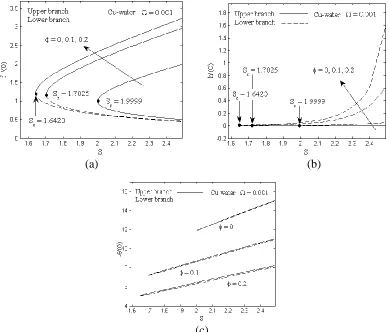
are given in the work of Oztop and Abu-Nada (2008). Figures 1 (a) to (c) present the effect of nanoparticle volume fraction on the variation of the skin friction coefficient
of x and y components, f(0)and
(0)
h and the local Nusselt number (0) with suction parameter for Cu-water nanofluid when 0.001. It is found that
the magnitude of the skin friction
coefficients for both components increase
with an increment in the value of . The fact that the presence of nanoparticles in the base fluid will accelerate the fluid motion
due to the collision between the
nanoparticles and base fluid particle. Thus, decreasing the momentum boundary layer thickness and consequently, increasing the skin frictions at the surface. Furthermore, the opposite trend is observed for the local Nusselt number as the increase. It should be noted that the critical values of suction seem to decrease as the increase.
(a) (b)
(c)
Figure 1. (a-c) Effect of nanoparticle volume fraction on the skin friction coefficient of x and
Figures 2 (a) to (c) illustrate the influence of the rotation on the variation of the f(0),
(0)
h and (0) with suction parameter for
2
TiO when 0.2. From these figures, the magnitude of the f(0), h(0) and
(0)
are noticed to increase when the
values of the rotation increase. However, the dual solutions exist when 0.001 for
2.0564, c
S while beyond this limit no
solutions exist. Sc is the critical value of suction for which Equations (8)-(10) have no solutions. It is worth mentioning that increasing the rotation in the flow reduces the momentum boundary layer thickness. Consequently, increases both the skin friction coefficients of x and y components on the wall.
(a) (b)
(c)
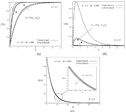
Figures 3 and 4 demonstrate the effects of the different nanoparticles and suction
the velocities of x andycomponents,
( ),
f h( ) and the temperature profiles ( ).
All the profiles are plotted to validate the numerical results obtained in the current study. It is shown that all profiles have satisfied the boundary conditions (11)
parameter on asymptotically with different patterns of graphs. As we noticed, the thickness of the boundary layer for the lower branch solution is always thicker than the upper branch solution.
(a) (b)
(c)
From this study, the stability of the dual solutions are identified using bvp4c function in MATLAB software. This analysis is conducted to know which of the upper or lower branch solution is linearly stable by depending on the sign of the smallest
eigenvalues obtained. The unknown
eigenvalue is introduced in Equation (23) and to determine the values of , the linear eigenvalue problems given in Equations (28)-(30) subjected to the conditions (31) is being applied. Table 1 and 2 displays the smallest eigenvalues for different values
of the selected parameters of interest. From the tables, the positive value of represents an initial decay of disturbance and the flow is said to be stable for the upper branch solution. Meanwhile, the negative value of refers to an initial growth of disturbance and the flow is an unstable for the lower branch solution. The stable flow is always given a good physical meaning that can be realized.
(a) (b)
(c)
Table 1. Smallest eigenvalues for various values of and S when 0.1 for Cu-water nanofluid.
S Upper branch Lower branch
0.0 2.1 0.9921 -0.6365
2.2 1.1591 -0.6890
2.3 1.3277 -0.7328
0.001 2.1 0.9922 -0.0352
2.2 1.1593 -0.0211
2.3 1.3279 -0.0104
0.1 2.1 1.3905 -
2.2 1.5495 -
2.3 1.7131 -
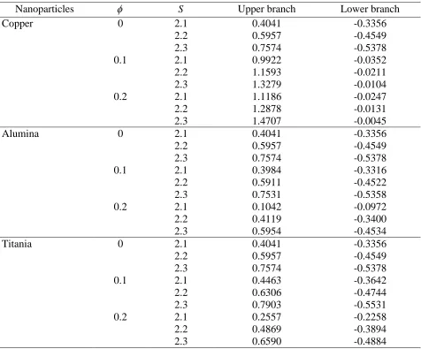
Table 2. Smallest eigenvalues for various values of and S using a different nanoparticles
when 0.001.
Nanoparticles S Upper branch Lower branch
Copper 0 2.1 0.4041 -0.3356
2.2 0.5957 -0.4549
2.3 0.7574 -0.5378
0.1 2.1 0.9922 -0.0352
2.2 1.1593 -0.0211
2.3 1.3279 -0.0104
0.2 2.1 1.1186 -0.0247
2.2 1.2878 -0.0131
2.3 1.4707 -0.0045
Alumina 0 2.1 0.4041 -0.3356
2.2 0.5957 -0.4549
2.3 0.7574 -0.5378
0.1 2.1 0.3984 -0.3316
2.2 0.5911 -0.4522
2.3 0.7531 -0.5358
0.2 2.1 0.1042 -0.0972
2.2 0.4119 -0.3400
2.3 0.5954 -0.4534
Titania 0 2.1 0.4041 -0.3356
2.2 0.5957 -0.4549
2.3 0.7574 -0.5378
0.1 2.1 0.4463 -0.3642
2.2 0.6306 -0.4744
2.3 0.7903 -0.5531
0.2 2.1 0.2557 -0.2258
2.2 0.4869 -0.3894
CONCLUSION
In this paper, the effect of the nanoparticles
volume fraction, rotation and suction
parameters on the fluid flow and heat transfer analysis of the rotating flow past a shrinking surface in nanofluid is investigated. The stability analysis is performed to identify the stability of the solutions obtained. Some discussions that can be made are as follows:
Dual solutions exist when the values of rotation are small enough, says
0.001
for Sc 2.0564 and beyond
this limit no solutions exist for TiO . 2
The highest values of heat transfer occur for Cu compared to Al O and 2 3
2
TiO due to it has higher thermal conductivity than others.
The upper branch solution is stable and physically realizable compared to the lower branch solution.
Increasing the rotation parameter gives rise the magnitudes of the skin friction coefficients and the local Nusselt number.
Increasing the nanoparticles volume
fraction parameter leads to an increase in the skin friction coefficients, while the opposite trend is found for the local Nusselt number.
ACKNOWLEDGEMENT
The authors gratefully acknowledged the financial support received from Ministry of Higher Education Malaysia in the form of
Fundamental Research Grant Scheme
(FRGS/1/2018/STG06/UPM/02/4/5540155) and Putra Grant GP-IPS/2018/9667900 from Universiti Putra Malaysia.
REFERENCES
Bachok, N., Ishak, A., & Pop, I. (2010). Boundary-layer flow of nanofluids over a moving surface in a flowing
fluid. International Journal of
Thermal Sciences, 49:1663-1668.
Bachok, N., Ishak, A., & Pop, I. (2012). Unsteady boundary-layer flow and heat transfer of a nanofluid over a permeable stretching/shrinking sheet.
International Journal of Heat and
Mass Transfer, 55:2102-2109.
Choi, S. U. S. (1995). Enhancing thermal
conductivity of fluids with
nanoparticles. ASME Publication,
231:99-105.
Das, K., Duari, P. R., Pop, I., & Kundu, P. K. (2014). Nanofluid flow over an
unsteady stretching surface in
presence of thermal radiation.
Alexandria Engineering Journal,
Hafidzuddin, E. H., Nazar, R., Arifin, N. M., & Pop, I. (2015). Stability analysis of unsteady three-dimensional viscous
flow over a permeable
stretching/shrinking surface. Journal
of Quality Measurement and Analysis,
11:19-31.
Harris, S. D., Ingham, D. B., & Pop, I. (2009).
Mixed convection boundary-layer
flow near the stagnation point on a vertical surface in a porous medium: Brinkman model with slip. Transport
Porous Media, 77: 267-285.
Mahapatra, T. R. & Nandy, S. K. (2011). Stability analysis of dual solutions in stagnation-point flow and heat transfer over a power-law shrinking surface.
International Journal of Nonlinear
Sciences, 12: 86-94.
Merkin, J. H. (1985). On dual solutions occurring in mixed convection in a
porous medium. Journal of
Engineering Mathematics,
20:171-179.
Nadeem, S., Rehman, A., & Mehmood, R. (2014). Boundary layer flow of rotating two phase nanofluid over a
stretching surface. Heat Transfer
Asian Research, 45:285-2
Najib, N., Bachok, N., & Ari_n, N. M. (2016). Stability of dual solutions in
boundary layer flow and heat transfer
over an exponentially shrinking
cylinder. Indian Journal of Science and Technology, 9:1-6.
Naramgari, S. & S ulochana, C. (2016). MHD
flow over a permeable
stretching/shrinking sheet of a
nanofluid with suction/injection.
Alexandria Engineering Journal,
55:819-827
Othman, N. A., Yacob, N. A., Bachok, N., Ishak, A., & Pop, I. (2017). Mixed convection boundary-layer stagnation point flow past a vertical stretching/ shrinking surface in a nanofluid.
Applied Thermal Engineering,
115:1412-1417.
Oztop, H. F. & Abu-Nada, E. (2008). Numerical study of natural convection
in partially heated rectangular
enclosures filled with nanofluids. International Journal of Heat Fluid Flow, 29:1326-1336.
Reddy, C. R., Murthy, P. V. S. N., Chamkha, A. J., & Rashad, A. M. (2013). Soret effect on mixed convection flow in a nanofluid under convective boundary condition. International Journal of Heat and Mass Transfer, 64:384-392.
Rosca, N. C. & Pop, I. (2014). Unsteady boundary layer flow of a nanofluid past a moving surface in an external
uniform free stream using
Buongiorno’s model. Computers and Fluids, 95:49-55.
Sharma, R., Ishak, A., & Pop, I. (2014).
Stability analysis of
magnetohydrodynamic
stagnation-point flow toward a
Weidman, P. D., Kubitschek, D. G., & Davis, A. M. J. (2006). The effect of transpiration on self-similar boundary layer flow over moving surfaces. International Journal of Engineering Sciences, 44:730-737.
Yasin, M. H. M., Ishak, A., & Pop, I. (2017). Boundary layer flow and heat transfer past a permeable shrinking surface embedded in a porous medium with a second-order slip: A stability analysis.
Applied Thermal Engineering,