ABSTRACT
This study addresses the issue of how modern information systems such as the geographic information system can help investment and managerial
decisions on real estate location. Specifically, this work is a case study of the
city of Manchester in the United Kingdom. Thematic maps are created for four districts within Manchester using socio-economic variables provided
by the Office of National Statistics. One of the two districts that demanded
the largest real estate average price is found to be associated with fewer
claimants for council tax benefits, fewer houses in the highest council tax
band, more people in good health, higher professional and skilled work force,
fewer people living on state benefits, and more green space. The other area demanding the highest average price is identified with having few people living on state benefits, and it comes only second to the best area in terms of green space. The study also examines the causal relationships identified in
the case study for the entire city of Manchester. The average annual prices
of four property types within Manchester (flats, semi-detached, terraced, and
detached) are regressed against changes in employment, household income,
inflation, and council tax. Flats’ prices are found to be the most sensitive to changes in income, as flats are the most affordable for real estate buyers.
Keywords: geographic information system, socio-economic variables, real estate
COMBINING GIS TECHNIQUES AND
SOCIO-ECONOMIC VARIABLES IN
THE REAL ESTATE DECISION-MAKING
PROCESS
M. F. Omran1
Hamed Ahmed Al-Marwani2
1College of Business
Qatar University, Doha, Qatar
2Qatar Fertilizer Company (QAFCO), Doha, Qatar
ARTICLE INFO
Article History :
Received : 25 November 2014
INTRODUCTION
Real estate located within a radius of a closely linked network of rails, roads, supermarkets, schools, and hospitals automatically attracts a sizable number of investors, as they feel more comfortable with the low investment risk. However, the real estate industry does not only consist of risk-averse investors but also risk-seeking investors who search for undeveloped and
virgin areas for investment. Risk seekers become the first to reap the financial benefits when the land develops over time. The question is how one can
identify a location that has the potential to achieve a substantial rate of return. Given this problem, the geographic information system (GIS) may help identify potential real estate locations. It can also help in management across functions, such as site planning, asset management, and market analysis. With the emergence of GIS, both spatial (location attributes) and non-spatial (socio-economic attributes) data can be managed simultaneously
to conduct better analysis and a more efficient decision-making process
(Li, Kong, Pang and Yu, 2003). Finding a real estate location that can have a positive net present value for the investor is an important question that GIS can help to address.
Fujiwara and Campbell (2011) discussed the link between an individual’s well-being and the health of the adjoining locality. Location or neighbourhood preference is not constant over time. Location is about identifying the best space or site that matches clients’ preferences. Therefore, location is one of the most important factors determining the value of real estate. Socio-economic factors include neighbourhood-established status, demographical tendencies, employment rate, major employment possibilities, household income, and council tax bracket. The importance of socio-economic factors when it comes to real estate location decision can never be ignored.
investment location issue using GIS and socio-economic variables obtained
from the Office of National Statistics (ONS) of the United Kingdom. Specifically, it concentrates on the city of Manchester in the United Kingdom
as a case study. The methodology can be easily expanded to cover other cities within the UK. Manchester was chosen because it is the second most populous conurbation behind London according to the ONS (2011).
A conurbation is formed when cities and towns expand sufficiently that
their urban areas join up with each other. Manchester was selected rather
than London as the latter has more foreign influences than the former. These foreign influences will make modeling more difficult as more international
factors have to be studied.
This paper is organized in seven sections. Section One presents the introduction. Section Two gives the literature review. Section Three
discusses how maps of real estates can be built on the basis of specific
geographic features. Section Four indicates how thematic maps can be created using GIS combined with socio-economic factors, as provided by the ONS. Section Five presents a case study of four selected districts within Manchester. Section Six discusses the causal modelling of Manchester, where real estate prices by property type are modelled using the
socio-economic factors identified in Section Five. Section Seven concludes the study with the finding that casual factors are important in the case study
of Manchester.
LITERATURE REVIEW
GIS is designed to categorically manage and analyze spatial relationships. Goodchild (1992) and Densham and Goodchild (1989) outlined how GIS could be utilized for various applications, including risk management. Thrall and Marks (1993) described the ability of the tool to study the spatial aspect of real estate decisions. Marks, Stanley, and Thrall (1994) provided guidelines for evaluating GIS software for the analysis of real estate. Previous research has underlined the importance of using GIS in real estate, but none has come up with a model that combines spatial and non-spatial data to choose optimal locations for real estate investments
Donlon (2007) reported that the precision of both spatial and non-spatial data improves the reliability of GIS analysis. With the increasing demand of GIS data in the planning profession, spatial data have become very important. The spatial data selection function includes a set of variables for particular locations from a spatial database (Fik, Sargent and Swett, 2005).
Real estate investment is a heterogeneous type of investment (Brown, 1997). Although market factors are important in determining the ups and downs in the market, the returns are also dependent on many other factors such as type of tenant, age of property, location, socio-economic parameters, and condition of the neighbourhood. Breedon and Joyce (1993)
found a positive significant relationship between real estate prices and
explanatory variables, such as earnings, disposable income, demography, rate of repossessions by lenders, and stock of dwellings. Breedon and Joyce (1993) also concluded that investment in residential units is linked to mortgage lending. Fujiwara and Campbell (2011) highlighted the importance of the link between an individual’s well-being and the health of the adjoining locality. Denzer (2005) found that a GIS addition to a business
decision-making process enhances the efficiency of decisions made. GIS is
particularly well suited for real estate practitioners, whose main criterion is “location”.
Weber (2001) discussed the basics of GIS and how it could be used for the valuation of real estate. Cowley (2007) observed that most research on using GIS technology in relation to property markets is dedicated to the sector of mass appraisal for rating and taxing purposes. However, the importance of socio-economic factors in real estate location decisions can never be ignored. The present study uses GIS to improve existing methodologies such as the ring study, drive time, and gravity models. Real estate market analysts usually rely on the ring study and drive time analysis (Fik, Sargent and Swett, 2005). In the ring study, circles are drawn around the real estate unit. The area of the circle gradually increases until it covers
a specified set of attributes or desired number of customers. The drive time
between areas considers such factors as customers’ willingness to travel, multiple modes of transportation, and consumer preferences. A variety of
of linking an analytical database to a spatial component such as locality. This linking advantage is what distinguishes GIS from other alternatives, such as the ring study, drive time and gravity models.
MAPPING REAL ESTATE INVESTMENT LOCATIONS
USING GIS
The use of GIS in the real estate domain is measured by the availability of consistent information. With the help of GIS, comparable data with
specific characteristics can be selected. Risk can be reduced through initial identification and visualization of the localities according to their
corresponding socio-economic factors. GIS helps to map relationships among demographics, household income of a particular location, and investment in real estate (De Man, 1998). It combines location and socio-economic data to create thematic maps that show a wide range of data related to population, housing and economic deprivation, and council tax claimant, among others.
GIS maps consist of points, lines, and polygons (Marks, Stanley and Thrall, 1994 and Podor, 2010). A layer can be a point, a polygon or a line.
A line can be defined as a shape having length and direction but no area,
and it connects at least two points or geographic coordinates. Examples of a line are roads or railways. A point is a digital representation of a place that has location, but it is too small to have an area or length on a particular scale, such as a city on a world map or a building on a city map. A polygon
has geometry, and it is significantly larger than a point on the map scale.
two adjacent districts, Higher Blackley (M001) and Blackley (M002), provide nearness of two localities. The one in Stanley Grove (M020) and the one in South Wythenshawe (M050) provide basis for comparison with the ones in the north.
CAUSAL RELATIONSHIP, SOCIO-ECONOMIC FACTORS
AND THEMATIC MAPS
A real estate project can fail not because it does not provide value but because it does not correspond to what the buyers are looking for. The basic objective of qualitative factors on buyers’ preferences is to ensure robustness of decision-making. Brereton, Clinch, and Ferreira (2008) analyzed the relation between an individual’s well-being and the adjoining environment and found that staying in public housing leads to a negative mindset and decreased individual satisfaction. Living in a deprived area has a direct effect on life satisfaction (Dolan, Peasgood and White, 2008; Abraham, Sommerhalder and Abel, 2010). Thrall (2002) found evidence that success in real estate investment is dependent on the success in identifying the location of a successful real estate asset.
Real estate buyers may make decisions using compensatory rules. They choose key features, rank competing real estates in each feature, and select the real estate with the maximum score. The alternative to compensatory rules is non-compensatory rules, in which all the essential features are not summed up. Some important determinant feature sways the decision toward a particular real estate choice (Alpert, 1971).
The personality of an individual can be a criterion that affects one’s investment in real housing choices. A risk seeker would invest in a property
in an undervalued location and reap the benefits when the neighbourhood
starts to improve. Changes in personal attitudes, lifestyle, and tastes tend
to influence individual preferences for real estate. Market analysts should
not only consider census but must also consider the behavioral changes and motivations of individuals (Rabianski, 1995).
of understanding the price behavior of real estate units, as it can explain price change under different market scenarios, such as boom and bust. Podor (2010) discussed the importance of tax attached to the unit. People tend to estimate the annual maintenance of the unit through this tax band. Moreover, the tax band helps people identify the status of the locality, i.e.,
whether affluent people or people living on state benefits reside in that
locality. Fujiwara and Campbell (2011) and Podor (2010) discussed how crime and safety might affect neighbourhood status and create a great impact on real estate price. Dolan, Peasgood, and White (2008) found that a key parameter for life satisfaction is neighbourhood status. Rabianski (1995) concluded that a major element for life satisfaction is the access to green
space. Podor (2010) considered basic education as a factor that influences
people’s decisions in buying or selling a real estate unit. Brereton, Clinch, and Ferreira (2008) found that people with the same ethnic race tend to live in the same locality. Brereton, Clinch, and Ferreira (2008), Thrall (2002), Fujiwara and Campbell (2011), and Podor (2010) indicated the importance of the proximity of basic facilities to the units people want to buy. Among these facilities are hospitals, schools, community center, police station, post
office, and railway stations.
From the ONS database, we are able to group the socio-economic causal factors into their corresponding domains, which can be related to real estate values. The database used in this paper is for 2011, and it uses seven domains to paint a broad picture of an area to determine the surrounding conditions. The data on the seven domains are available at www.ons.gov. uk. The domains measure the general “health” and determine the successful locality across the city.
The seven domains are as follows:
1. Crime and Safety 2. Economic Deprivation 3. Health Care
4. Housing
5. Personal Consumer Debt 6. Social Grade
The inputs for these domains are updated at least annually. These domains are used as guidelines for mapping real estate investment opportunities. They are explained as follows.
Crime and Safety
ONS Statistics holds data on vital offenses from the crime series
record of the Home Office. The data are used to analyze crime trends at
the local level. In the crime and safety database, data on both crime (theft,
burglaries, harassment, arson attack, etc.) and safety (fire-related issues) are
grouped together. The records under the crime component are suppressed because they are considered sensitive. This domain is not used because
its data are considered sensitive and can only be released upon official
request. However, the main rationale behind this domain is that a post code investment will be more desirable if its crime rate is lower than that of another competitive post code.
Economic Deprivation
This domain is a count of housing benefit (council tax benefit) claimed
by the residents. The ONS collects the data from the Department of Work and Pensions. It can help the real estate developer in locating his/her targeted
clientele. For example, an area with a low count of council tax benefit may
be suitable for an above average housing development project.
Health Care
The ONS holds data on the general health of residents living in different areas in the United Kingdom. Data are categorized into good health of the residents, fairly good health of the residents, and not good health of the residents. This information can help the real estate developer in locating appropriate projects.
Housing
The ONS holds data on the following housing relevant items:
and the number and percentage of properties that have corresponding standard council tax bands.
2. Average house price.
3. Housing stock that is composed of household spaces and occupied household spaces. This item is not used because it has no available data in the ONS website.
This domain can provide vital statistics on the target house price and its related council tax band.
Personal Consumer Debt
The ONS data show in sterling pounds the range of average personal consumer debts per person for different districts. Debts related to individual businesses or commercial concerns are not included. A district characterized
by a higher average consumer debt and classified as dominated by a high
percentage of unemployment excludes high-end real estate projects for this district. An affordable real estate project with options for land or real estate swaps is recommended.
Social Grade
The ONS data show individuals aged 16 and over who live in
households according to their corresponding social economic classification:
higher and intermediate managerial professionals, supervisory professionals, skilled manual workers, semi-skilled and unskilled worker, and on state
benefit-unemployed. This domain is important in the planning stage of real
estate investment location. As explained in the personal debts domain, social grades and personal debts are important drivers of real estate investments.
Environment
These domains contain the data of each explanatory variable per respective district. These attributes are then linked to the area maps using the ArcGIS software to generate thematic maps of each district. A thematic map is a type of map especially created to show a particular theme related
to a specific geographic area. These maps can help visualize physical,
social, political, cultural, economic, sociological, or any other aspects of a district. Figure 1 shows an example of a thematic map of district 001 Manchester bordered in yellow. The different color schemes map the number
of claimants in the receipt of housing or council tax benefit.
Figure 1: Map Showing the Total Number of Claimants in the Receipt of Housing Benefit or Council Tax Benefit1
Different maps can be created for each district with regard to one of the seven socio-economic domains provided by the ONS. The legend values of the maps are used to conduct the empirical analysis in Section Five of the causal relationship between real estate price and socio-economic explanatory variables.
EMPIRICAL ANALYSIS OF THE CAUSAL
RELATIONSHIPS
The objective of this section is to establish casual relationships between real estate prices and explanatory variables, such as socio-economic dimensions. The districts chosen for the analysis, as explained in Section Four, are Higher Blackley (M001), Blackley (M002), Stanley Grove (M020), and South Wythenshawe (M050). The seven domains used as explanatory variables
are defined and discussed in Section Four. These domains are:
1. Crime and Safety 2. Economic Deprivation 3. Health Care
4. Housing
5. Personal Consumer Debt 6. Social Grade
7. Environment
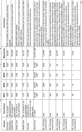
Domain Sub-domain M001 M002 M020 M050 Manchester Conclusion
Economic Deprivation No. of people claiming tax benefit
1590
1600
1775
1820
64,800
M001 and M002 are best with less people claiming benefits.
Health Care
No. of people in good health
4374
4700
4454
4380
253,665
M002 is best in terms of more people in good health.
Health Care
No. of people in fairly good health
1869
1872
1766
2008
90,039
M050>M002>M001>M020 M002 is second to M050 in terms of people in fairly good health. M001 is third.
Health Care
No. of people in not so good health
1127 1145 1122 1234 49,1 15
Inconclusive since numbers are very close to each other
.
Housing
Dwelling Stock (total number of real estate units)
3836
4177
3705
3821
217,085
M002 has most stocks in line with its advance position in terms of economic deprivation and health care.
House Price
(in GBP)
80,000 GBP 85,000 GBP 85,000 GBP 84,000 GBP
1,25,000 GBP
M002 demands the highest average real estate price in accordance with its advance position in economic well- being and health care. Other factors should contribute to the house price in M020.
No. of houses under B and
A units 3121 2999 3107 3534 1,29,861
M002 has fewer houses in the tax
A band. Opportunities
for high-end real estate developments may be available in M002.
No. of houses under B and B
units 355 635 471 217 35,280
M002 has more houses in band B than in other bands. Same conclusion as above. Opportunities for high-end developments in tax band
A may be available in M002.
No. of houses under Band C
units 209 423 107 62 29,797
M002 has more houses in band C than in other bands. Same conclusion as above. Opportunities for high-end development in tax band
A may be available in M002.
No. of houses under Band D
units 107 94 15 7 14,221
M002 is second to M001, as it has more houses in band D than in other bands. Same conclusion as above. Opportunities for high-end developments in tax band
A
may be available in M002.
No. of houses under Band E
units 26 19 1 1 5139
M002 is second to M001, as it has more houses in band E than in other bands. Same conclusion as above. Opportunities for high-end developments in tax band
A
may be available in M002.
Table 1: Neighbourhood Index Domain Comparison
Among M001, M002, M020 and M050
No. of houses under Band F units 14 3 1 0 1940
M002 is second to M001, as it has more houses in band F than in other bands. Same conclusion as above. Opportunities for high-end developments in tax band
A
may be available in M002.
No. of houses under Band G
units 2 4 2 0 748
Numbers are too small to be conclusive.
No. of houses under Band H
units 2 0 1 0 99
Numbers are too small to be conclusive.
Personal Consumer Debt
(in GBP)
2508 GBP 1539.93 GBP 2630.71 GBP 1398.68 GBP
1836.53 GBP
M050>M002>M001>M020 Personal consumer debts are low in M050, followed by M002. However
, the two are not far from each other
,
especially in comparison with M001 and M020.
No. of higher professionals
people 524 655 462 342 48,523
M002 has the largest higher professional community
.
This finding supports the earlier conclusion that the area may be suitable for high-end developments, which come under band
A council tax.
No. of higher professionals
people 838 1422 1090 737 35,690
M002 has the largest higher skilled worker community
.
This finding supports the earlier conclusion that the area may be suitable for high-end developments, which come under band
A council tax.
No. of skilled workers
people 1332 888 638 1652 66,574
M002 ranks second in having low semi-skilled workers.
No. of semi- skilled and unskilled Workers
people 1422 1494 1444 1098 78,233
With the exception of M050, distinguishing among M001, M002, and M020 is difficult.
No. of supervisory professionals
people 1533 1406 1528 1685 65,788
M002>M020>M001>M050 M002 has fewer people living on state benefits than the other areas.
This finding supports the earlier conclusion
that the area may be suitable for high-end developments.
Environment
(green space, thousand square meters)
1126.20
970.44
638.69
385.28
40,556.32
M001>M002>M020>M050 M002 ranks second to M001 in terms of green space. However
, M001 and M002 are not far away from each
other
N.B.: Council Tax Band Details: Band A: Up to 40,000 GBP, Band B: 40,001 GBP–52,000 GBP, Band C: 52,001 GBP–68,000 GBP, Band D: 68,001 GBP–88,000 GBP, Band E: 88,001 GBP–120,00 GBP, Band F: 120,001 GBP–160,00 GBP, Band G: 160,001 GBP–320,00 GBP, and Band H: 320,001 GBP and above
The conclusions in the last column in Table 1 show that M002 and M020 have the highest average real estate price of GBP 85,000. M002 is
identified as the best location among the four areas (M001, M002, M020, and M050). M002 has fewer claimants for council tax benefits, fewer
houses in high council tax band A, more people in good health, higher
professional and skilled work force, fewer people living on state benefits,
higher average house price, and more green space than M020 and M050. M002 seems like an attractive place for real estate investment, as it provides a better environment for individuals’ well-being. M020 is the second best area in terms of green space and the lowest in personal consumer debts. It
is also second to M002 in terms of having less people on benefits. These
conclusions establish a pattern that should be tested; i.e., real estate prices are positively correlated with higher income, fewer council tax claimants, good health, and green space.
CAUSAL MODELING OF MANCHESTER
Section Five hypothesizes positive causal relationships between real estate price changes on the one hand and higher income, fewer council tax claimants, good health, and green space on the other hand. Data are collected
on the employment rate, household income, inflation, and council tax from 1998 to 2013. The data are from the Official Labor Market Statistics, UK
(NOMIS: www.nomisweb.co.uk), and they are available on an annual basis
only. Real estate price averages by property type (flats, semi-detached,
77
Combining GIS Techniques and Socio-Economic Variables
The following regression is used:
yt = α + β1X1+ β2X2 + β3X3 + β4X4 + ut, (1)
where
yt = change in real estate price,
14
averages by property type (flats, semi-detached, terraced, and detached) are used. The annual
data for average real estate prices by property type within Greater Manchester from quarter 1 of
1998 to quarter 1 of 2013 are obtained from the Land Registry of the UK
(
www.landregistry.gov.uk
). The Land Registry Database covers all house prices of Greater
Manchester.
The following regression is used:
y
�=
α � β
�X
�+
β
�X
�+
β
�X
�+
β
�X
�+
u
�,(1)
where
y
�= change in real estate price,
�����������,
α
= constant,
β
�, β
�, β
�, β
�= parameter estimates,
X
�= change in employment,
X
�= change in income,
X
�= inflation,
X
�= change in council tax,
u
t= residual term assumed to be normally distributed with mean zero and variance one.
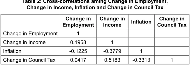
The cross-correlations of the explanatory variables are presented in Table 2. The cross
correlations are examined to avoid multicollinearity. Multicollinearity will not be a problemas
long as the cross-correlation between two variables is less than 0.7. Both variables can be
included as explanatory variables.
Table 2: Cross-correlations amingChange in Employment,Change in Income, Inflation, and Change in Council Tax
Change in
employment Change in Income Inflation Council Tax Change in
Change in Employment 1
Change in Income 0.1958 1
Inflation -0.1225 -0.3779 1
Change in Council Tax 0.0417 0.5183 -0.3313 1
None of the correlations reported in Table 2is larger than 0.70,thus indicating no risk of
multicollinearity. The highest positive correlation is between change in income and change in
council tax. The regression is run for the all property types.The results areshown in Table 3
Table 3: Regression of Real Estate Property Price on Changes from Previous ,
α = constant,
β1, β2, β3, β4= parameter estimates,
x1 = change in employment, x2 = change in income,
x3 = inflation,
x4 = change in council tax,
ut = residual term assumed to be normally distributed with mean zero and variance one.
The cross-correlations of the explanatory variables are presented in Table 2. The cross correlations are examined to avoid multicollinearity. Multicollinearity will not be a problem as long as the cross-correlation between two variables is less than 0.7. Both variables can be included as explanatory variables.
Table 2: Cross-correlations aming Change in Employment, Change in Income, Inflation and Change in Council Tax
Change in
Employment Change in Income Inflation Council TaxChange in
Change in Employment 1
Change in Income 0.1958 1
Inflation -0.1225 -0.3779 1
Change in Council Tax 0.0417 0.5183 -0.3313 1
Table 3: Regression of Real Estate Property Price on Changes from Previous Years in Employment, Income, Inflation, and Council Tax
Property
Types and t test for Co-efficient
Change in Employment
Co-efficient and t test for Change
in Income
Co-efficient and t test for Change in Inflation
Co-efficient and t test for Change
in Council Tax
Co-efficient and t test for Constant
Adjusted
R-Squared testF
Semi-Detached 0.368(0.25) (0.23)2.676 (0.86)1.354 (0.03)0.043 -0.046(-0.63) .0159 0.217 Detached 0.406(0.14) (1.64)3.96 (-0.76)-2.393 -1.979(-0.72) 0.073(0.5) 0.042 0.378 Flats (-0.87)-1.469 3.421**(2.48) (0.17)0.312 (-0.71)-1.118 -0.007(-0.08) 0.160** 0.216 Terraced (-0.76)-1.657 (1.59)2.833 (1.17)2.740 (0.48)0.980 -0.082(-0.76) 0.049 0.365
***, ** and * indicate significance at the 1%, 5%, and 10%, respectively
The table indicates non-significant relationships between the price
changes for each property type and the explanatory variables, except for
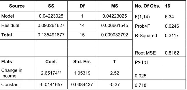
the real price changes for flats and changes in income. Table 4 shows the regression of price changes for flats as a dependent variable and the changes
in income as the explanatory variable.
Table 4: Regression Analysis between Flat Prices and Change in Income
Source SS Df MS No. Of Obs. 16
Model 0.04223025 1 0.04223025 F(1,14) 6.34
Residual 0.093261627 14 0.006661545 Prob>F 0.0246
Total 0.135491877 15 0.009032792 R-Squared 0.3117
Root MSE 0.8162
Flats Coef. Std. Err. T P> I t I
Change in
Income 2.65174** 1.05319 2.52 0.025
Constant -0.0141657 0.0384437 -0.37 0.718
***, ** and * indicate significance at the 1%, 5%, and 10%, respectively
Price changes for flats are significantly positively correlated at 5% with
change in income. A positive increase in income leads to a positive increase
is 31%, which indicates that 31% of the variation in prices of flats can be
explained by the variation in household income.
SUMMARY
The study addresses the issue of how modern information systems such as GIS can help in investment and managerial decisions with regard to real estate location. This work is a case study of the city of Manchester in the United Kingdom. Thematic maps are created for four districts of Manchester using socio-economic variables provided by the ONS. One of the two areas, which demands the largest real estate average price, is
found to be associated with fewer claimants for council tax benefits, fewer
houses in high council tax band A, more people in good health, higher
professional and skilled work force, fewer living on state benefits, and more green space. These factors are consistent with those considered to influence
an individual’s well-being. The other area demanding the highest average
price is identified to have few people living on state benefits, and it comes
only second to the best area in terms of green space. This study examines
the causal relationships identified in the case study of Manchester. Annual data were collected for employment, income, inflation, and council tax
from 1998 to 2013. Multiple regressions were estimated for price changes for each of the four property types as dependent variables, and for change
in employment, change in income, inflation, and change in council tax as independent variables. The only significant relationship was observed between price change for flats and changes in income. However, data were
available on an annual basis and for a relatively short time period only. Accordingly, the sample size was small, and changes were less frequent to capture the underlying causal relationships. Nevertheless, the case studies of the four areas in Manchester provide us with the clear insight that causal models are important in determining real estate prices.
ACKNOWLEDGEMENTS
The authors would like to acknowledge the helpful comments they received
from anonymous reviewers and from the participants of the Asian Pacific
which was hosted by Chulalongkorn University in Bangkok, Thailand from October 27 to October 30, 2014.
REFERENCES
Abraham, A., Sommerhalder, K. and Abel, T. (2010) “Landscape and well-being: a scoping study on the health-promoting impact of outdoor environments”, International Journal of Public Health 55, 1; 59-69.
Alpert, Mark I. (1971) “Identification of Determinant Attributes”, Journal
of Marketing Research, 8, 184-191.
Armstrong, Martin A. (2009) “A Forecast For Real Estate”, http:// armstrongeconomics.com/wp-content/uploads/2012/03/a-forecast-for-real-estate-111509.pdf. Website was last visited on May 3rd 2014.
Breedon, F.J. and Joyce, M.A.S. (1993) “House prices, arrears and possessions: a three equation model for the UK”, Bank of England Working Paper Series No. 14.
Brereton, F., Clinch, J.P. and Ferreira, S. (2008) “Happiness, geography and the environment”, Ecological Economics, 65, 2; 386-396.
Brown, G.R. (1997) “Reducing the dispersion of returns in U.K. real estate portfolios”, Journal of Real Estate Portfolio Management, 3, 2; 129:140.
Cowley, M (2007) “Project Viability Studies and Market Forecasts - A Survey of Property Developers”, Urban Developer, 1; 24.
Densham, Paul J., and Michael F. Goodchild (1989) “Spatial Decision Support Systems: A Research Agenda”, Proceedings GIS/LIS 1989, 707:716. Orlando, FL: American Society for Photogrammetry and Remote Sensing.
Denzer R. (2005) “Generic integration of environmental decision support systems-state-of-the-art”, Environmental Modelling and Software, 20, 10; 1217:1223.
Dolan, P., Peasgood, T., and White, M. (2008) “Do we really know what makes us happy? A review of the economic literature on the factors associated with subjective wellbeing”, Journal of Economic Psychology, 29; 94:122.
Donlon K.H. (2007) “Using GIS to Improve the Services of a Real Estate Company” http://www.gis.smumn.edu/GradProjects/DonlonK.pdf Website was last visited on May 3rd 2014.
Fik T. C. Sidman, B. Sargent, and R. Swett. (2005) “A Methodology for Delineating A Primary Service Area For Recreational Boaters Using A Public Access Ramp: A Case Study Of Cockroach Bay”, The Florida Geographer, 36; 23-40.
Fujiwara, D., and Campbell, R. (2011) “Valuation Techniques for Social
Cost-Benefit Analysis: Stated Preference, Revealed Preference and
Subjective Well-Being Approaches”, https://www.gov.uk/government/ uploads/system/uploads/attachment_data/file/209107/greenbook_ valuationtechniques.pdf Website last visited on May 3rd 2014.
Goodchild, Michael F. (1992) “Geographical Information Science”, International Journal of Geographical Information Systems, 6, 1; 31-45.
Li, H., Kong, C.W., Pang, Y.C. and Yu, L. (2003) “Internet-based geographical information systems system for E-commerce application in construction material procurement”, Journal of Construction Engineering and Management, 129, 689-97.
Marks, A., C.Stanley, and G.Thrall, (1994). “Criteria and Definitions for
the Evaluation of Geographic Information System Software for Real Estate Analysis”, Journal of Real Estate Literature, 2; 227:244.
Rabianski, Joseph (1995) “Market analyses and Appraisals”, Real Estate Issues, Winter; 45-49.
Thrall, G. and A. Marks (1993) “Functional Requirements of a Geographic Information System for Performing Real Estate Research Analysis”, Journal of Real Estate Literature, 1, 1; 49:61.
Thrall, G.I. (2002) “Business Geography and New Real Estate Market Analysis”, Oxford Press: Oxford.