Simulation modeling of the sensitivity analysis of differential effects of the intrinsic growth rate of a fish population: its implication for the selection of a local minimum

(1)

https://dx.doi.org/10.22161/ijaems.4.1.7 ISSN: 2454-1311

Simulation modeling of the sensitivity analysis of

differential effects of the intrinsic growth rate of a

fish population: its implication for the selection of

a local minimum

Nwachukwu Eucharia C.

1

_{, Ekaka-a Enu-Obari N.}

2

_{, Atsu Jeremiah U.}

3

1_{Department of Mathematics and Statistics, University of Port Harcourt, Port Harcourt, Nigeria} 2_{Department of Mathematics, Rivers State University, Nkpolu,Port Harcourt, Nigeria} 3_{Department of Mathematics/Statistics, Cross River University of Technology, Calabar, Nigeria.}

Abstract—The vulnerability of the differential effects of the intrinsic growth rates of the fish population on the uncertainty analysis can only be controlled by using the mathematical technique of a sensitivity analysis that is called a local minimum selection method based on a Matlab numerical scheme of ordinary differential equations of order 45 (ODE 45). The quantification of the p-norms sensitivity analysis depends on the application of the 1-norm, 2-1-norm, 3-1-norm, 4-1-norm, 5-1-norm, 6-norm and infinity-norm. In the context of this study, the best-fit intrinsic growth rate of fish population with a small error has occurred when its value is 0.303 which minimizes the bigger sensitivity values previously obtained irrespective of the p-norm sensitivity values. The novel results which we have obtained have not been seen elsewhere. These results are fully presented and discussed in this study.

Keywords— Uncertainty analysis, differential effects, p-norms sensitivity analysis, intrinsic growth rate, local minimum, ODE45.

I. INTRODUCTION

Following Ekaka-a et al (2012), sensitivity analysis is a measure of the resultant effect due to a variation of a model parameter value on the model solution trajectories. It a mathematical tool to enhance model validation and prediction. On the other hand, on-going debate among many researchers including Palumbi (1999), Sumali (2002), Pitchford (2007) and Bohnsack (1993) has shown that marine reserve is not only economically important but can also serve as a tool for equitable management of biodiversity especially in the context of fisheries.Kar and Charkraborty (2009), in their work titled marine reserves and its consequences as a fisheries management tool

described a prey-predator type fishing model with prey dispersed in a 2-patch environment, one of which is called a free fishing zone and another, a protected zone. Their main method of investigation uses the simulation process. One key contribution from their work states that prey-predator dichotomy do not matter when implementation of a reserve is considered. Their second result shows that reserves will be most effective when coupled with fishing effort controls in adjacent fisheries. Despite the fact that marine reserves and its consequences can be effectively utilized as a fisheries management tool, it is still an open research problem that these authors did not consider the technique of sensitivity analysis which is vital numerical incentive in a decision process that can lead to an effective fisheries management.

It remains an open problem to study the differential effects of varying the intrinsic growth rate of the fish population on the uncertainty analysis using a one-at-a-time sensitivity analysis Hamby 1995. It is against this background that we propose to use ODE45 RungeKutta numerical scheme with initial condition 2 4 2 over a period of fifty (50) weeks to study the differential effects of the intrinsic growth rate of fish population on the sensitivity analysis that is indexed by seven classifications of the sensitivity analysis, namely: 1-norm error analysis, 2-1-norm error analysis, 3-1-norm error analysis, 4-norm error analysis, 5-norm error analysis, 6-norm error analysis and infinity-6-norm error analysis.

(2)

which describes the prey-predator fisheries management model. Hence, we modify the model as follows:

𝑑

𝑑𝑡𝑥(𝑡) = 𝑟1𝑥(𝑡) − 𝛽1𝑥(𝑡)

2_{− 𝜇1𝑥(𝑡) 𝑦(𝑡) −}𝜎

𝛼𝑥(𝑡) +

𝜎

𝛼−1𝑦(𝑡) − 𝑚𝑥(𝑡)𝑧(𝑡) (3.1) 𝑑

𝑑𝑡𝑦(𝑡) = 𝑟2𝑦(𝑡) − 𝛽2𝑥(𝑡)𝑦(𝑡) − 𝜇2𝑦(𝑡) 2₊𝜎

𝛼𝑥(𝑡) −

𝜎

𝛼−1𝑦(𝑡) − 𝑛𝑦(𝑡)𝑧(𝑡) − 𝑞𝐸𝑦(𝑡) (3.2) 𝑑

𝑑𝑡𝑧(𝑡) = 𝑟3𝑧(𝑡) − 𝑟3𝛾𝑧(𝑡)2

𝑥(𝑡)+𝑦(𝑡)

(3.3) 𝑥(0) = 2, 𝑦(0) = 4, 𝑧(0) = 2

(3.4)

In this model, x(t) represents the fish stock in the reserved area at time t, y(t) is the fish stock in the unreserved area at time t, z(t) is the biomass density of the predator species at time t. 𝑟1is the intrinsic growth rate of fish stock x, 𝑟2is the intrinsic growth rate of fish stocky, 𝑟3 is the intrinsic growth rate of the predator species, 𝛾 is the equilibrium ratio between prey biomass and predator biomass, m is maximum relative increase in predation to the reserved area or simply put, the contribution of z to inhibit the growth of fish stock (x) in the reserved area, n is maximum relative increase in predation to the unreserved area or simply put, the contribution of z to inhibit the growth of fish stock (y) in the unreserved area. The predation terms are therefore defined as mxz and nyz with respect to fish stocks in the reserved and unreserved area respectively. In addition, 𝜎 is the mobility coefficient, 𝛼 is the size of the reserved area, 1 − 𝛼 is the size of the unreserved area, q is catch ability coefficient, E is effort applied for harvesting fish population in the unreserved area.

Further mathematical interpretation can be invoked to describe the interaction of the three equations. In equation

(3.1), 𝑑

𝑑𝑡𝑥(𝑡) = 𝑟1𝑥(𝑡) shows that without interaction with other y and z species, the x population grows unboundedly as time increases. The same observation is made for the y

and z populations. This is mathematically correct but practically unrealistic, hence the need for the interaction between the species. We can deduce the following interpretations term by term:

𝛽1𝑥(𝑡)2_{is the contribution of fish stock in the reserved area} to inhibits its original exponential growth.

𝜇1𝑥(𝑡) 𝑦(𝑡)is the contribution of fish stock in the unreserved area to inhibit the growth of fish population in the reserved area.

𝜎

𝛼𝑥(𝑡)is the effect of the ratio of the migration rate/mobility coefficient to the size of the reserve area to inhibit the growth of fish stock in the reserved area

𝜎

𝛼−1𝑦(𝑡)is the effect of the ratio of the migration rate/mobility coefficient to the size of the unreserved area to enhance the growth of fish stock in the reserved area 𝑚𝑥(𝑡)𝑧(𝑡)is the contribution of z to inhibit the growth of fish stock on the reserve area

𝛽2𝑥(𝑡)𝑦(𝑡)is the contribution of fish stock in the reserved area to inhibit the growth of fish population in the unreserved area.

𝜇2𝑦(𝑡)2is the contribution of fish stock in the unreserved area to inhibits its original exponential growth.

𝜎

𝛼𝑥(𝑡)is the effect of the ratio of the migration rate/mobility coefficient to the size of the reserve area to inhibit the growth of fish stock in the unreserved area

𝜎

𝛼−1𝑦(𝑡)is the effect of the ratio of the migration rate/mobility coefficient to the size of the unreserved area to inhibit the growth of fish stock in the unreserved area 𝑛𝑦(𝑡)𝑧(𝑡)is the contribution of the predator biomass to inhibit the growth of fish stock on the unreserved area 𝑞𝐸𝑦(𝑡)is the contributed effect of the fishing effort and Catchability coefficient to inhibit the growth of the fish stock in the unreserved area.

𝑟3𝛾𝑧(𝑡)2

𝑥(𝑡)+𝑦(𝑡)is equilibrium ratio on the fish stocks in the reserved and unreserved area due to activities of the predator biomass.

For the purpose of our mathematical analysis, the value for model parameter r is the same value for: 𝑟1, 𝑟1, 𝛽1, 𝛽2, 𝜇1, 𝜇2and 𝑠 = 𝑟3. In addition, we shall adopt the model parameter values as proposed by Kar and Charkraborty (2009): 𝑟 = 0.3, 𝜎 = 0.2, 𝑚 = 1, 𝑛 = 1, 𝑞 = 0.0025, 𝑠 = 0.1, 𝛾 = 0.95, 𝐸 = 95.

III. METHOD OF ANALYSIS

The core part of the algorithm which we have utilized to calculate the sensitivity of a model parameter is hereby described by the following steps which has also been implemented in the work of Ekaka-a et al (2013):

Step I: identify and code the control system of given model equations of continuous non-linear first order ordinary differential equation in which the model parameter is not varied. For the purpose of this analysis, the three solution trajectories are denoted by 𝑥, 𝑦,and 𝑧.

(3)

first order ordinary differential equation in which the model parameter is varied one-at-a-time. In this case, the three solution trajectories are denoted by 𝑥𝑚, 𝑦𝑚, and 𝑧𝑚.

Step III : code an appropriate Matlab program using ODE Runge-Kutta scheme to execute the program in Step I and Step II. With the initial conditions and a time range, the execution program will produce the solution trajectories for the programs in step I and step II.

On the execution program, specify the difference between the solution trajectories of the codes in step I and step II as 𝐹1= 𝑥 − 𝑥𝑚, 𝐹2= 𝑦 − 𝑦𝑚 and 𝐹3= 𝑧 − 𝑧𝑚

Step IV: Use the execution program to calculate the 1-norm, 2-1-norm, 3-1-norm, 4-1-norm, 5-1-norm, 6-norm and infinity-norm for the three solution trajectories of the control model equations and similarly for the solution trajectories for the difference between the solution trajectories. For example, for the x and xm solution trajectories which assume precise data points such as xj and

xmj, where the subscript j takes on the values of 1, 2, 3, 4, …,n, the 1-norm for the x solution trajectory is defined as the sum of the absolute values of x1, x2, x3, up to the nth point xn. In the same manner, the 2-norm of the x1 solution trajectory is defined by the positive square root of the sum of the squares of absolute values of x1, x2, x3, up to the nth point xn. Similarly, the 3-norm for the x solution trajectory is defined as the sum of the absolute values (cubed) of x1,

x2, x3, up to the nth point xn. The 4-norm for the x solution trajectory is defined as the sum of the absolute values (to fourth power) of x1, x2, x3, up to the nth point xn. The 5-norm for the x solution trajectory is defined as the sum of the absolute values (to fifth power) of x1, x2, x3, up to the nth point xn. The 6-norm for the x solution trajectory is defined as the sum of the absolute values (to sixth power) of

x1, x2, x3, up to the nth point xn. The infinity norm for xm is defined by the maximum value of the set of the absolute values of x1, x2, x3, up to the nth point xn. The same procedure holds for the calculation of 1-norm, 2-norm, 3-norm, 4-3-norm, 5-3-norm, 6-norm and infinity norm for y and z solution trajectories.

Step V: In the execution program, calculate the difference between the solution trajectories of the control model equation and the varied model equation by 𝐹1= 𝑥 − 𝑥𝑚, 𝐹2= 𝑦 − 𝑦𝑚 and 𝐹3= 𝑧 − 𝑧𝑚 for the given range of data points when j = 1, 2, 3, 4, …, n such that the difference between the solution trajectories of the control model equations and the varied model equations would be 𝐹1= 𝑥𝑗− 𝑥𝑚𝑗, 𝐹2= 𝑦𝑗− 𝑦𝑚𝑗 and 𝐹3= 𝑧𝑗− 𝑧𝑚𝑗.

For the purpose of this analysis, we will also calculate the 1-norm, 2-norm, 3-norm, 4-norm, 5-norm, 6-norm and

infinity norm of 𝐹1,𝐹2 and 𝐹3. For example, 1-norm of F1 will be the sum of the absolute values of the data points (𝑥1− 𝑥𝑚1), (𝑥2− 𝑥𝑚2), (𝑥3− 𝑥𝑚3),(𝑥4− 𝑥𝑚4), …, (𝑥𝑛− 𝑥𝑚𝑛) where 𝑥1 and 𝑥𝑚1 stand for the first data point of x solution trajectory and the first data point of the modified 𝑥𝑚 solution trajectory respectively. 𝑥2and𝑥𝑚2 stand for the second data point of x solution trajectory and the second data point of the modified 𝑥𝑚 solution trajectory respectively and so forth. The 1-norm of F2 will be the sum of the absolute values of the data points (𝑦1− 𝑦), (𝑦2− 𝑦𝑚2), (𝑦3− 𝑦𝑚3),(𝑦4− 𝑦𝑚4), …, (𝑦𝑛− 𝑦𝑚𝑛) where 𝑦1 and 𝑦𝑚1 stand for the first data point of y solution trajectory and the first data point of the modified 𝑦𝑚 solution trajectory respectively. 𝑦and𝑦𝑚2 stand for the second data point of y solution trajectory and the second data point of the modified 𝑦𝑚 solution trajectory respectively and so forth. Similarly, the 1-norm of F3 will be the sum of the absolute values of the data points (𝑧1− 𝑧𝑚1), (𝑧2− 𝑧𝑚2), (𝑧3− 𝑧),(𝑧4− 𝑧𝑚4), …, (𝑧𝑛− 𝑧𝑚𝑛) where 𝑧1 and 𝑧𝑚1 stand for the first data point of z solution trajectory and the first data point of the modified 𝑧𝑚 solution trajectory respectively. 𝑧2and𝑧𝑚2 stand for the second data point of z solution trajectory and the second data point of the modified 𝑧𝑚 solution trajectory respectively and so forth. The 2-norm, 3-2-norm, 4-2-norm, 5-2-norm, 6-norm and infinity norm can similarly be calculated for the differences of three solution trajectories 𝐹1,𝐹2 and 𝐹3.

Step VI: To calculate the cumulative percentage effect of variation of a chosen model parameter one-at-a-time when other parameters are fixed on each solution trajectory. For x

solution trajectory, we will calculate the following values: (1-norm of 𝐹1 divided by the 1-norm of x) multiplied by 100; (2-norm of 𝐹1 divided by the 2-norm of x) multiplied by 100; (3-norm of 𝐹1 divided by the 3-norm of x) multiplied by 100; (4-norm of 𝐹1 divided by the 4-norm of

x) multiplied by 100; (5-norm of 𝐹1 divided by the 5-norm of x) multiplied by 100; (6-norm of 𝐹1 divided by the 6-norm of x) multiplied by 100 and (infinity-norm of 𝐹1 divided by the infinity-norm of x) multiplied by 100. To calculate the percentage cumulative effect of variation of a model parameter one-at-a-time when other parameters are fixed on y solution trajectory, we will calculate the following values: (1-norm of 𝐹2 divided by the 1-norm of y) multiplied by 100; (2-norm of 𝐹2 divided by the 2-norm of

(4)

the 6-norm of y) multiplied by 100 and (infinity-norm of 𝐹2 divided by the infinity-norm of y) multiplied by 100. To calculate the percentage cumulative effect of variation of a model parameter one-at-a-time when other parameters are fixed on z solution trajectory, we will calculate the following values: (1-norm of 𝐹3divided by the 1-norm of z) multiplied by 100; (2-norm of 𝐹3 divided by the 2-norm of

z) multiplied by 100; (3-norm of 𝐹3 divided by the 3-norm of z) multiplied by 100; (4-norm of 𝐹3 divided by the 4-norm of z) multiplied by 100; (5-norm of 𝐹3 divided by the 5-norm of z) multiplied by 100; (6-norm of 𝐹3 divided by the 6-norm of z) multiplied by 100 and (infinity-norm of 𝐹3 divided by the infinity-norm of z) multiplied by 100. Due to the unstable values of the 1-norm, 2-norm, 3-norm, 4-norm, 5-norm, 6-norm and infinity-norm specifications, we adopt to use a compact value for related percentage values of these norms. For example, the cumulative percentage value of 1-norm sensitivity in terms of the difference in solution trajectories involves the sum of the 1-norm values due to 𝐹1 solution trajectory, 1-norm values due to 𝐹2 solution trajectory and 1-norm values due to 𝐹3 solution trajectory. The same procedure can be followed to calculate the cumulative percentage values for norm, 3-norm, 4-3-norm, 5-3-norm, 6-norm and infinity-norm

sensitivities in terms of 𝐹1 solution trajectory, 𝐹2 solution trajectory and 𝐹3 solution trajectory.

The cardinal points of sensitivity analysis results interpretation are:

 the parameter which when varied a little and produces the biggest cumulative effect on the solution trajectories is called a most sensitive parameter. And it is highly uncertain. This by implication will attract error in prediction and thus require further validation.

 the parameter which when varied a little andproduces lower or least sensitivity values is called a less or least sensitive parameter and requires lesser validation.

Method for Best-fit parameter value selection

In order to select the best-fit parameter value for each model parameter, we recommend that

 At 100% variation, the coordinates of the solution trajectories have same values, sums, squares and square roots = 0. Therefore, the norm values at 100% are zero.

The Local minimum value is selected at a point where the smallest norm value occurs before or after the 100% variation.

IV. RESULTS AND DISCUSSION

On the application of the define method of analysis, we hereby present and discuss the following results:

Table.1: sensitivity analysis results for model parameter r

r 1-norm 2-norm 3-norm 4-norm 5-norm 6-norm ∞-norm

0.0030 143.9520 78.8284 82.0093 66.2747 56.624 50.6594 29.8099 0.0060 143.1933 78.4409 81.6042 65.9501 56.348 50.4130 29.6754 0.0090 142.3997 78.0321 81.1766 65.6070 56.056 50.1521 29.5334 0.0120 141.5698 77.6010 80.7256 65.2447 55.747 49.8763 29.3837 0.0150 140.7023 77.1468 80.2503 64.8624 55.421 49.5850 29.2259 0.0180 139.7958 76.6685 79.7499 64.4593 55.077 49.2776 29.0605 0.0210 138.8491 76.1654 79.2236 64.0350 54.715 48.9538 28.8879 0.0240 137.8610 75.6368 78.6706 63.5887 54.334 48.6131 28.7078 0.0270 136.8304 75.0818 78.0903 63.1201 53.934 48.2553 28.5200 0.0300 135.7565 74.4999 77.4821 62.6287 53.514 47.8800 28.3243 What do we learn from Table 1?

We have observed from table 1 that as the value of the model parameter r increases monotonically from 0.003 (approx) to 0.03 (approx), the 1-norm error data decreases monotonically from the value of 143.95 (approx.) to 135.76 (approx.), the 2-norm error data decreases monotonically from the value of 78.83 (approx.) to 75.50 (approx.), the 3-norm error data decreases monotonically from the value of 82.01 (approx.) to 77.48 (approx.), the 4-norm error data

(5)

On the basis of this present analysis we have observed that r

= 0.003 is associated with relatively higher uncertainty when compared to the value of r = 0.03 irrespective of the type of p-norm we have used to calculate the sensitivity analysis. Despite the observed uncertainty analysis results due to a one percent to ten percent variation of the intrinsic growth rate of the fish population, it is clear that the statistical range of the p-norm sensitivity values are listed as follows: the range of 1-norm statistical range is 8.19, the

range of 2-norm statistical range is 3.33,the range of 3-norm statistical range is 4.53,the range of 4-norm statistical range is 3.64,the range of 5-norm statistical range is 3.11,the range of 6-norm statistical range is 2.78 ,the range of infinity-norm statistical range is 1.49.

These bigger sensitivity values which indicate high uncertainty of the intrinsic growth rate of the fish population can be further minimized.

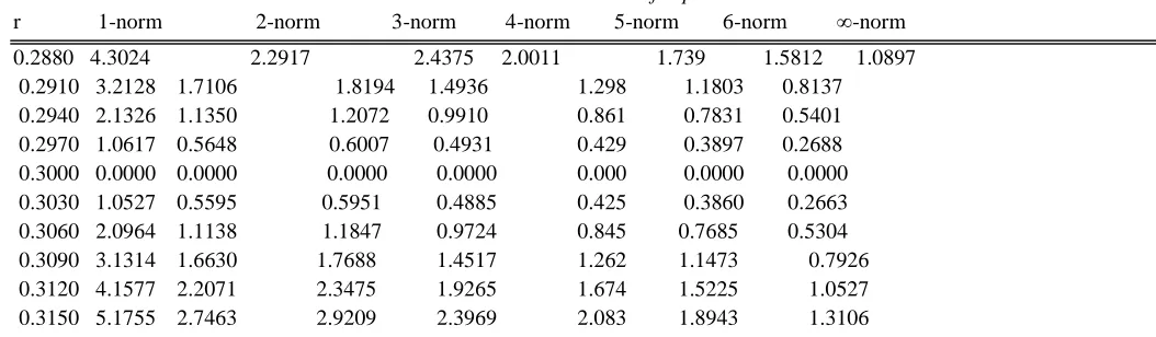
Table.2: local minimum resultsfor parameter r

r 1-norm 2-norm 3-norm 4-norm 5-norm 6-norm ∞-norm

0.2880 4.3024 2.2917 2.4375 2.0011 1.739 1.5812 1.0897 0.2910 3.2128 1.7106 1.8194 1.4936 1.298 1.1803 0.8137 0.2940 2.1326 1.1350 1.2072 0.9910 0.861 0.7831 0.5401 0.2970 1.0617 0.5648 0.6007 0.4931 0.429 0.3897 0.2688 0.3000 0.0000 0.0000 0.0000 0.0000 0.000 0.0000 0.0000 0.3030 1.0527 0.5595 0.5951 0.4885 0.425 0.3860 0.2663 0.3060 2.0964 1.1138 1.1847 0.9724 0.845 0.7685 0.5304 0.3090 3.1314 1.6630 1.7688 1.4517 1.262 1.1473 0.7926 0.3120 4.1577 2.2071 2.3475 1.9265 1.674 1.5225 1.0527 0.3150 5.1755 2.7463 2.9209 2.3969 2.083 1.8943 1.3106

What do we learn from Table 2?

Table 2 shows a result of the cumulative effect of 96 to 105 percent variation of model parameter r. At 100percent variation, there are no changes in the original and the varied solution trajectories, hence the zero values.

Observe that as the model parameter value increase monotonically from a low value of 0.2880 to 0.0000 corresponding to 100 percent variation and then increases monotonically to 0.3150 approximately in column I, the 1- norm sensitivity value decreased monotonically from a value of 4.30 to 0.0000 corresponding 100 percent variation and then increases monotonically to 5.18 approximately in column II, the 2- norm sensitivity value decreased monotonically from a value of 2.29 to 0.0000 corresponding 100percent variation and then increases monotonically to 2.75 approximately in column III, the 3- norm sensitivity value decreased monotonically from a value of 2.44 to 0.0000 corresponding 100percent variation and then increases monotonically to 2.92 approximately in column IV, the 4- norm sensitivity value decreased monotonically from a value of 2.00 to 0.0000 corresponding 100percent variation and then increases monotonically to 2.40 approximately in column V, the 5- norm sensitivity value decreased monotonically from a value of 1.74 to 0.0000 corresponding 100percent variation and then increases monotonically to 2.08 approximately in column VI, the 6-

norm sensitivity value decreased monotonically from a value of 1.58 to 0.0000 corresponding 100percent variation and then increases monotonically to 1.90 approximately in column VII, the infinity- norm sensitivity value decreased monotonically from a value of 1.09 to 0.0000 corresponding 100percent variation and then increases monotonically to 1.31 approximately in column VIII.

The local minimum is selected at the greatest lower bound of the data points for each p-norm results. For instance, the local minimum value for model parameter r is 0.303 where 1-norm local minimum value = 1.0527, 2-norm local minimum value = 0.5595, 3-norm local minimum value = 0.0.5951, 4-norm local minimum value = 0.4885, 5-norm local minimum value = 0.4250, 6-norm local minimum value = 0.3860 and infinity-norm local minimum value = 0.2663.

V. CONCLUSION

(6)

model parameter values which we did not consider in this study in our future investigation.

REFERENCES

[1] E. N. Ekaka-a, N. M. Nafo, A. I. Agwu, (2012), Examination of extent of sensitivity of a mathematical model parameter of survival of species dependent on a resource in a polluted environment, International Journal of Information Science and Computer Mathematics, vol. 8, no 1-2, pp 1-8.

[2] EnuEkaka-a, Olowu, B. U., Eze F. B., Abubakar R. B., Agwu I. A., Nwachukwu E. C., (2013), Journal of Nigerian Association of Mathematical Physics, Vol 23, pp 177-182.

[3] Palumbi S. (1999). The ecology of marine protected areas: Working paper from the Department of Organismic and Evolutionary Biology, Harvard University.

[4] Rodwell L. D, Edward B. Barbier, Callum M. Roberts, Tim R. Mcclanahan (2002), A model of tropical marine reserve-fishery linkages. Natural Resource Modeling, 15(4).

[5] Sumalia U. (2002) Marine protected area performance in a model of the fishery. Natural Resource Modeling, 15(4).

[6] J. Pitchford, E.Codling, D. Psarra. Uncertainty and sustainability in fisheries.Ecological Modelling, 2007, 207: 286–292.

[7] Kar, T. and Chakraborty, K. (2009): Marine reserves and its consequences as a fisheries management tool, World Journal of Modelling and Simulation, (2009) 5(2), pp. 83-95.

[8] J. Bohnsack. Marine reserves: They enhance fisheries, reduce conflicts, and protect resources. Oceanus, 1993,63–71.