Performance Evaluation of ZigBee Transceivers using
Convolutional Coding Technique
Hikmat N. Abdullah
Information and Communication Engineering Department,
College of Information Engineering University of Al-Nahrain/
Baghdad
Tariq M. Salman
Department of Electrical Engineering, College of Engineering Al-Mustansiriya University/
Baghdad
Haider A.H. Alobaidy
Department of Electrical Engineering, College of Engineering Al-Mustansiriya University/
Baghdad
ABSTRACT
The aim of this paper is to evaluate the amount of improvement introduced in ZigBee transceivers when channel-coding methods are used. A MATLAB-Simulink model of the ZigBee transceiver that uses soft decision based Convolutional Coding (CC) at different code rates is proposed. It is observed from the simulation results that using convolutional coding in ZigBee transceiver gives better performance than the traditional ZigBee transceivers and that the convolutional code of code rate 1/8 gives the best performance as compared to other rates. In AWGN channel and at BER of 10-4, the maximum coding gains obtained over traditional system are 14dB and 13.5dB for OQPSK and BPSK (868-900MHz) based ZigBee respectively, while these gains are 23.5dB, 40.5dB and 19.5dB, 12.5dB in Rayleigh & Rician fading channels at the same BER respectively.
General Terms
Channel Coding, Performance.
Keywords
ZigBee transceivers, IEEE 802.15.4 standard, Wireless Sensor Networks (WSN), Soft decision based convolutional coding, MATLAB Simulink.
1.
INTRODUCTION
In early 2003, the IEEE STD 802.15.4 was ratified after many years of effort. This standard represented a significant break from the “bigger and faster” standards that the IEEE 802 organization continues to develop: instead of higher data rates and more functionality, this standard was to address the simple, low-data volume universe of control and sensor networks, which existed without global standardization through a miasma of proprietary methods and protocols [1]. The IEEE standard identifies and controls only the RF, PHY and Medium Access Control (MAC) layers, and there are variety of custom and industry-standards based networking protocols that can sit atop this IEEE stack. The standard states that wireless links can operate in the 2.4 GHz, the 915 MHz or the 868 MHz Industrial Scientific and Medical (ISM) bands. The standard allocates 16 channels in the 2.4 GHz band, 10 channels in the 915 MHz band, and only one channel in the 868 MHz band and that makes a total of 27 channels are allocated by this standard. Despite the fact that the standard devices can use any of these bands, the 2.4 GHz band is more common as it is certified in most of the countries worldwide [2].
ZigBee is a protocol that uses the IEEE STD 802.15.4 as a baseline and adds additional routing and networking functionality. It was developed by the ZigBee Alliance [3]. The Alliance has worked hard to provide a technology that takes best advantage of the robust IEEE STD 802.15.4 short-range wireless protocol. This is done by adding flexible mesh networking, strong security tools, well-defined application profiles, and a complete interoperability, compliance and certification program to ensure that the end products destined for residential, commercial and industrial spaces work well and network information smoothly [1]. The main function that was added to the core of IEEE STD 802.15.4 radio in the development of ZigBee protocol is mesh networking. Mesh networking is used in applications where data is to be sent between two points beyond the scope of coverage of the radio devices located in those points. This is solved in mesh networking by adding some radios in-between that are capable of forwarding any message to and from the intended radios [3].
2.
ZIGBEE RF TRANSCEIVER
INFRASTRUCTURE
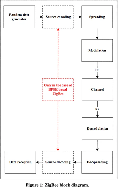
ZigBee can be Offset Quadrature Phase Shift Keying (OQPSK) based working in the 2.4GHz band or Binary Phase Shift Keying (BPSK) based working either in the 868MHz or in 900MHz band [12]. However, the block diagram of the ZigBee transceivers can be summarized as shown in Figure 1. In addition, the specification of ZigBee operating in each band can be summarized as shown in Table 1.
Figure 1: ZigBee block diagram.
Table 1: Specification of ZigBee in 2.4GHz, 868MHz, and 900MHz bands [12].
2.4GHz 868MHz 900MHz
Spreading method
16-array orthogonal
Binary DSSS
Binary DSSS
Chip rate 2Mcps 300kcps 600kcps
Modulation OQPSK BPSK BPSK
Bit rate 250kbps 20kbps 40kbps
Symbol rate 62.5ksps 20ksps 40ksps
Number of allocated channels
16 1 10
3.
CONVOLUTIONAL CODES (CC)
Convolutional codes are the most popular and widely used in most of the communication systems [13, 14]. The main feature enabled by CC is real time error correction. Convolutional codes are generated by passing a data sequence through a shift register, which has two or more sets of register taps each set terminating in a modulo-2 adder [13]. CC converts the entire data stream into one single codeword [14]. This codeword is produced by sampling the output of all the modulo-2 adders once per shift register clock period. It is called convolutional codes since the coder output is obtained by the convolution of the input sequence with the impulse response of the coder [13]. The encoded bits depend not only on the current ‘k’ input bits but also on past input bits. These codes are usually specified as (n, k, L) where n is the number of output bits from the coder, k is the number of input bits to the coder and L is the constraint length of the coder. The constraint length is used to calculate the number of memory stages or Flip-Flops used in the encoder [14]. The error correcting power is related to the constraint length, increasing with longer lengths of shift registers [13]. The constraint length can be expressed as [14]:……… Eq.1
Where is the number of memory elements.
Another important thing to understand is the generator polynomial of CC that specifies how the memory elements are linked to achieve encoder. These generator polynomials are usually found through simulation [14]. Some textbooks gives tables describing some convolutional codes including their code rate R (k/n), free distance of the convolutional code dfree, constraint length, and the generator polynomial. Figure 2
shows an example of (2,1,3) CC encoder structure and Table 2 shows the parameters of several convolutional codes. The convolutional code encoder can also be represented as a finite state machine and a tree diagram, trellis diagram, or a state transition diagram may represent the operation of the encoder [13, 14]. As for decoder, there may be three main types. These are based on sequential, threshold (majority logic) and Viterbi decoding techniques [13]. Out of these, the Viterbi decoding is the most popular one [13, 14].
Table 2: Parameters of several rate k/n convolutional codes [15, 16]
Code rate k/n
Constraint length L
Generator polynomial
G in octal dfree
1/2
3 [5 7] 5
4 [15 17] 6
5 [23 35] 8
8 [371 247] 10
14 [21675 27123] 17
1/3
3 [5 7 7] 8
4 [13 15 17] 10
5 [25 33 37] 12
8 [225 331 367] 16
14 [21645 35661 37133] 26
1/4
3 [5 7 7 7] 10
4 [13 15 15 17] 15
14 [21113 23175 35527 35537] 36
1/5
3 [7 7 7 5 5] 13
4 [17 17 13 15 15] 16
8 [257 233 323 271 357] 28
12 [7725 6671 5723 5321 4317] 38
1/6
3 [7 7 7 7 5 5] 16
4 [17 17 13 13 15 15] 20
8 [253 375 331 235 313 357] 34
1/8
3 [7 7 5 5 5 7 7 7] 21
8 [275 275 253 371 331 235 313 357] 45
13
[17623 16365 15221 14331 13277 12467
11275 10473]
64
2/3 4 [236 155 337] 7
3/5 2 [35 23 75 61 47] 5
4.
HARD AND SOFT DECISION
DECODING [14]
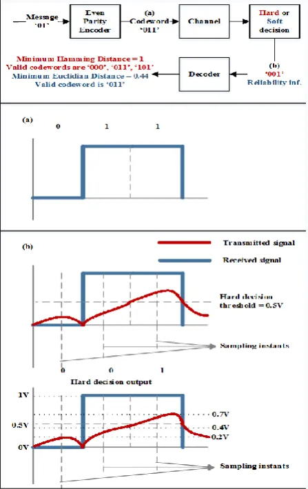
As it is known, any receiver input signal is in analog form. Sampling, quantization and coding is used by the receiver to convert the signal back to digital domain. However, in the case of hard decision receiver the quantizer quantizes the sampled values in the sampling step into either ‘0’ or ‘1’. This is the simplest quantization method that uses only two levels. The hard decision receiver simply decides whether the received bit is zero or one. This is usually achieved by using a certain threshold. For example, if a two bits message encoded using say ‘even parity encoder’. In this case, four possible
codewords are generated and they are ‘000’, ‘001’, ‘101’, ‘110’. Now assuming that the message ‘01’ is transmitted over a communication channel. Then the hard decision block shown in Figure 3 predicts whether the received bits are zero or one according to its predefined threshold that is 0.5V in this example, i.e. any value less than 0.5 will be detected as ‘0’ otherwise it will be detected as ‘1’. The received codeword is then compared with all possible codewords mentioned previously and the Hamming Distance (HD) is computed for each case. The codeword that gives the minimum HD is selected which makes some confused decisions such as in the example that gives three possible solutions.
As for the case of soft decision decoding, the received codeword is also compared with all possible codewords and then the Euclidian Distance is computed instead of HD. The codeword that gives the minimum Euclidian Distance is selected. This improves the decision making process by supplying additional reliability information, i.e. calculated Euclidian Distance or log-likelihood ratio.
In soft decision the quantization step is not of two levels as in hard decision instead, it is of multilevel for example 8-levels, i.e. each bit is represented by 3bits. In AWGN channel, the 8-level quantization improves the performance in terms of SNR by 2dB compared to two level quantization and by 2.2dB in the case of infinite quantization. As a result, the 8-level quantization is preferred most times since the difference in performance is short compared to infinity quantization systems.
5.
IMPLEMENTATION OF
TRADITIONAL ZIGBEE
TRANSCEIVER
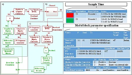
ZigBee transceivers can either be OQPSK based with data rate of 250kbps or BPSK based with data rate of 20kbps or 40kbps. Figures 4 and 5 show the overall implemented ZigBee transceivers. However, for simplicity design process is divided into three parts: ZigBee transmitter, channel model and ZigBee receiver.
5.1
The transmitter design
The OQPSK based ZigBee transmitter design as well as its blocks configuration is shown in Figure 4a. It includes four basic components (or blocks), these are:
Random data generation: A “Bernoulli Binary Data generator” available in the MATLAB/Simulink library is used to generate the input data with data rate of 250kbps. The configuration parameters of this block is shown in the right side of Figure 4.
PN sequence generation: The required 32-Bit chip sequence of chip rate 2Mcps is generated using “PN sequence generator” block available in the MATLAB Simulink library.
Spreading process: First both data generated and the PN Sequence output need to be converted to Bipolar using “unipolar to bipolar” block. The spreading is simply done by multiplying the binary data and PN chips using “product” block. The resulting output is converted back to unipolar data using “bipolar to unipolar” block.
Modulation: The spread data is modulated with “OQPSK baseband modulation” block. At this level, the data is ready for transmission through channel to its destination.
As for BPSK based transmitter, the same steps are followed except that generated data are differentially encoded using “differential encoder” block and the data rate can be either 40Kbps for 900MHz band or 20kbps for 868MHz band. After spreading, the spread data are modulated using “BPSK modulator” block as shown in Figure 5a.
5.2
Channel Model
The transmission channel models can be of three types as shown in Figure 6:
AWGN channel: This is the simplest channel model. It is achieved using the “AWGN” block in the Simulink library. It is very important to setup the parameters of AWGN block correctly such as number of bits per symbol (which is two in the case of OQPSK based ZigBee and one in the case of BPSK based ZigBee), input Power and the type of noise, i.e. SNR, Eb/No or
Es/No.
Rayleigh multipath fading channel: In this channel model, both Rayleigh and AWGN channels are used together with Maximum Likelihood Sequence Estimate (MLSE) equalizer. The MLSE equalizer block uses the Viterbi algorithm to equalize the linearly modulated signal through a dispersive channel. The block processes input frames and outputs the MLSE of the signal, using an estimate of the channel modeled as a Finite Impulse Response (FIR) filter. The test is made for indoor channel environment. In such environment, the ZigBee
nodes are fixed and for this reason, the Doppler spectrum is assumed to be near zero. Figure 6a depicts the Simulink implementation of this channel type. In this channel, the multipath fading is verified with path delays starting from one path delay up to six path delays for “ITU indoor channel model” and “Winner indoor channel model”. However, for simplicity in this paper only ITU channel model is presented with fixed three path delays [10-9, 15×10-9, 20×10-9] and average path gains of [-2.4 dB, -1.9 dB, -8.1 dB] respectively.
Rician multipath fading channel: As in Rayleigh channel, this channel model uses both Rican and AWGN channels together with MLSE equalizer. Figure 6b depicts the Simulink implementation of this channel with its parameter specifications. As in Rayleigh channel, only ITU channel models have been used. The parameters of ITU indoor hospital channel model in the case of Rician channel are of path delays [10-9, 10×10-9,
25×10-9] and average path gains of [0 dB, -15.7 dB, -10.5 dB]respectively. Note that the main difference between Rayleigh and Rician channels is that Line-Of-Sight (LOS) component is considered in the case of Rician channel model. Furthermore, K-factor is of 5 dB for ITU hospital channel model.
5.3
The receiver design
The OQPSK based ZigBee receiver design as well as its blocks configuration is shown in Figure 4c. It includes three basic steps, these are:
Demodulating the received signal using “OQPSK demodulator” block.
Generating the same PN sequence generated at transmitter side.
De-spreading: Before conversion of both demodulated data and PN sequence output, some synchronization process must occur. Synchronization is necessary to get rid of any possible delay in the received signal and to match the PN sequence with the start of data so that after product operation the same sent data is recovered with some delay at the start of reception which can be ignored.
As for BPSK based receiver design, the same steps are followed except that at demodulation step a “BPSK demodulator” block is used instead of OQPSK demodulator. Furthermore, the final output need to be differentially decoded using “Differential Decoder” block as shown in Figure 5c.
6.
IMPLEMENTATION OF CODED
ZIGBEE TRANSCEIVER
multipath fading channel, and Rician multipath fading channel.
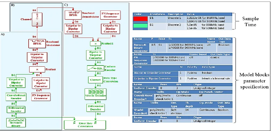
The channels specifications used here are the same as in the case of uncoded system. The difference lies in the setup of AWGN block and MLSE equalizer block. For AWGN block, the symbol time is changed and it is computed using:
T_sym=No.of bits per symbol×Sample time×Code rate … Eq.2
As for MLSE equalizer, the difference is in the channel coefficients and the output buffer size that must be the same as the buffer size of the input data to the channel.
Figure 4: Simulink implementation of Traditional (uncoded) OQPSK based ZigBee block diagram
a) ZigBee Transmitter. b) Channel Model. c) ZigBee Receiver
Figure 5: Simulink implementation of Traditional (uncoded) BPSK based ZigBee block diagram.
Figure 6: Simulink implementation of the used channel models.
Rayleigh channel and equalizer. b) Rician channel and equalizer. c) AWGN Channel
Figure 7: Simulink implementation of Coded OQPSK based ZigBee transceiver block diagram.
Figure 8: Simulink implementation of Coded BPSK based ZigBee transceiver block diagram.
a) Coded BPSK based ZigBee transmitter. b) Channel Model. c) Coded BPSK based ZigBee receiver
7.
SIMULATION RESULTS
This section discusses the results obtained from the designed ZigBee transceiver. The results can be categorized according to the channel model used during simulation into:
AWGN channel.
Rayleigh multipath fading channel.
Rician multipath fading channel.
7.1
ZigBee transceiver simulation results in
AWGN channel
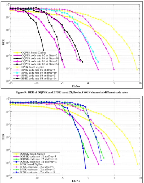
Figure 9 show the BER vs. Eb/No results obtained from
simulating the designed ZigBee transceivers with and without coding at different code rates starting from 1/2 up to 1/8. It is clearly noticeable that the one using CC code of code rate 1/8 gives the best performance compared to others. At BER of 10-4, the coding gain is between 4.5dB and 14dB for OQPSK based ZigBee and between 4dB and 13.5dB for BPSK (868-900MHz) based ZigBee. Figure 10 compares the traditional ZigBee transceiver with the coded ZigBee at a fixed coding rate of 1/2 and varying constraint length and dfree. Note that at
BER of 10-4, the coding gain starts from 4.5dB for OQPSK based ZigBee and 4dB for BPSK based ZigBee, and then starts to raise up when a code of higher constraint length and dfree is used. However, CC of dfree=17 gives a coding gain of
6dB for OQPSK based ZigBee and of 6.5dB for BPSK based ZigBee.
From the previous results it is clear that the simulated models of OQPSK based ZigBee have a performance transition region that starts at BER of about 10-2 with Eb/No of -3dB. Similarly,
for BPSK based ZigBee performance transition starts at BER of about 10-2 with Eb/No of zero dB and this proves that the
performance of OQPSK based ZigBee is better than that of BPSK based ZigBee. Note that the performances of both
868MHz and 900MHz based ZigBee are very close to each other in AWGN channel. It is also clear from the previous figures that the performance starts to increase as the code rate increases. However, the coding gain obtained varies from 5dB to 12dB.
7.2
ZigBee transceiver simulation results in
Rayleigh multipath fading channel
Now that the difference in performance occurred due to the use of different CC is clear. The constraint length is fixed in all other simulations and equals 3 plus fixed codes of code rate 1/2, 1/4, and 1/8 are used. The test in this channel is taken to verify the effect of multipath fading on the performance of ZigBee module and the improvement achieved. Figure 11 shows the performance of OQPSK, BPSK (868MHz), and BPSK (900MHz) based ZigBee transceivers respectively in ITU indoor hospital channel model. At BER of 10-4, the coding gain is between 14dB and 23.5dB for OQPSK based ZigBee, 11.5dB and 40.5dB for BPSK (868MHz) based ZigBee, and between 12dB and 40dB for BPSK (900MHz) based ZigBee. In this channel the BPSK based ZigBee gives the worst performance in all simulated performance tests.7.3
ZigBee transceiver simulation results in
Rician multipath fading channel
Figure 9: BER of OQPSK and BPSK based ZigBee in AWGN channel at different code rates
Figure 11: BER of OQPSK and BPSK based ZigBee in Rayleigh channel based on ITU hospital channel model
8.
CONCLUSIONS AND FUTURE WORK
ZigBee based wireless sensor network is an important area of research. However, this research work has been done to improve the robustness of ZigBee transceivers against channel noise and fading. The following conclusions have been drawn after processing the results generated from computer simulations work:The use of convolutional coding in ZigBee transceiver gives the best performance compared to the traditional ZigBee transceivers. Using CC of code rate 1/8 gives the best performance compared to other CC code rates when combined with ZigBee transceivers. At the same code rate, increasing constraint length and dfree increases the system performance as
well.
Future work involves two suggestions. Implementing the proposed improved ZigBee transceiver using FPGA. Regarding the good results obtained from the use of CC, it can be suggested to use other channel codes such as Turbo Code, etc.
9.
REFERENCES
[1] J. Zheng and M. Lee, "A Comprehensive Performance Study of IEEE 802.15.4," Sensor Network Operations, IEEE Press, Wiley Interscience, pp. 218-237, 2006.
[2] A. R. Raut and D. L. G. Malik, "ZigBee: The Emerging Technology in Building," International Journal on Computer Science and Engineering (IJCSE), vol. 3, no. 4, pp. 1479-1484, 2011.
[3] White Paper, "Demystifying 802.15.4 and ZigBee," [Online]. Available: http://www.digi.com/.
[4] S. Lanzisera and K. Pister, "Theoretical and Practical Limits to Sensitivity in IEEE 802.15.4 Receivers," in 14th IEEE International Conference on Electronics, Circuits and Systems, Marrakech, 2007.
[5] B. M. Khammas, "Design Neural Wireless Sensor Network Using FPGA," Eng. & Tech. Journal, vol. 30, no. 9, pp. 1641-1661, 2012.
[6] F. L. Lewis, "Wireless Sensor Networks," in Smart Environments: Technologies, Protocols, and Applications, New York, John Wiley & Sons, Inc., Hoboken, New Jersey, 2004, pp. 11-46.
[7] S. Gill, N. Suryadevara and S. Mukhoopadhyay, "Smart Power Monitoring System Using Wireless Sensor Networks," in Sixth International Confrence on Sensing Technology (ICST), Kolkata, 2012.
[8] N. K. Suryadevara, S. C. Mukhopadhyay, S. D. T. Kelly and S. P. S. Gill, "WSN-Based Smart Sensors and Actuator for Power Management in Intelligent Buildings," IEEE/ASME TRANSACTIONS ON MECHATRONICS, vol. 20, no. 2, pp. 1-8, 2014.
[9] L. C. Huang, H. C. Chang, C. C. Chen and C. C. Kuo, "A ZigBee-based monitoring and protection system for building electrical safety," Energy and Buildings, vol. 43, no. 6, pp. 1418-1426, 2011.
[10] H. K. Choudhari, A. A. Waoo, P. S. Patheja and S. Sharma, "Performance Evaluation of ZigBee Using Multiple Input Single Output (MISO) Architecture in the Secured Environment," International Jornal of Innovative Technology and Exploring Engineering (IJITEE), vol. 2, no. 6, pp. 36-44, 2013.
[11] Y. V. Varshney and A. K. Sharma, "Comparitive Analysis of OQPSK and MSK Based Zigbee Tranceiver Using MATLAB," International Journal of Advanced Research in Computer Science and Software Engineering, vol. 3, no. 6, pp. 948-956, 2013.
[12] S. Farahani, ZigBee Wireless Networks and Tranceivers, Elsevier, 2008.
[13] l. A. Glover and P. M. Grant, Digital Communication, England: Prentice Hall, 2010.
[14] M. Viswanathan, Simulation of Digital Communication Systems Using Matlab, Mathuranathan Viswanathan at Smashwords, 2013.
[15] J. G. Proakis and M. Salehi, Digital Communications, New York: McGraw-Hill, 2008.