Energy Efficiency Optimization in Wireless Sensor
Network Using Proposed Load Balancing Approach
Sukhkirandeep Kaur
Research Scholar, National Institute of Technology, Srinagar, India.
[email protected]
Roohie Naaz Mir
Professor, National Institute of Technology,Srinagar,India.
[email protected]
Published Online: 03 October 2016
Abstract – Advancement in MEMS technology, networking and embedded microprocessors have led to the development of a new generation of a Wireless Sensor Network (WSN) that can operate in unattended and harsh environment depending upon application. WSN consist of large number of power-conscious devices called sensor nodes that detect and observe any physical phenomenon and can be used in a wide range of applications. Underlying topology plays an important role in the performance of the Wireless Sensor Network. Depending upon the application, deployment is performed either deterministically or randomly. WSN suffers from a lot of issues that includes energy conservation, scalability, latency, computational resources and communication capabilities. Energy efficiency is critical issue in Wireless Sensor Networks as nodes are equipped with limited power supply and nodes that bypass most of the traffic deplete their energy faster that leads to decreased network lifetime. Incorporating clustering in the network improves scalability, increase energy efficiency and reduces redundancy. A new clustering approach for WSN has been discussed that includes load balancing and improves energy efficiency by precise selection of CH's. Analysis and simulation results demonstrate the effectiveness of the proposed approach.
Index Terms – Wireless Sensor Networks (WSN), Base Station (BS), Clustering, Load Balancing (LB).
1. INTRODUCTION
Wireless sensor network (WSN) consists of large number of low power autonomous devices called sensor nodes or motes that work in collaboration to retrieve data based on application domain. With the advancement in MEMS technology and ability to sense any physical phenomenon, sensor devices are used in numerous applications like healthcare, military applications, surveillance and monitoring etc. Different applications have different network requirements and these applications plays an important role in our day to day life. For example Health Monitoring System for the Elderly and Disabled has been developed in [1] that monitors health activities remotely and in case of any emergency, immediate help can be provided. Applications of WSN for Disaster
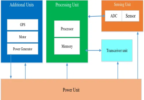
Management is discussed in [2] that throws a light on how WSN architecture can be used in handling disaster management situations. Main components of a sensor node consists of sensing unit that senses any physical phenomenon, processing unit that performs different computations and communication subsystem that exchanges information between different nodes. Architecture of sensor node is presented in Figure 1.
Additional Units Processing Unit Sensing Unit
Transceiver unit
Power Unit
Motor GPS
Power Generator
Processor
Memory
ADC Sensor
Figure 1 Sensor Node Architecture
WSN is entirely application dependent and based on the application, different deployment strategies, protocols and algorithms are designed for WSN. Data collection process in WSN can be continuous, event driven and query based [3]. Based on data model used, sensor nodes collect data and transmit to the Base Station in single hop or multi hop communication. Base-station can be stationary or mobile, depending upon the network and it connects sensor network to internet or existing infrastructure.
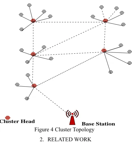
nodes, their transmission range, distance between neighbors, type of routing paths, type of communication etc. For monitoring and surveillance applications, deterministic deployment is preferred as these applications demand more QoS requirements and these requirements can be ensured through careful planning of node densities and fields of view and thus network topology can be established at setup time[4]. For applications that are deployed in hostile environments such as forest fire detection, disaster recovery etc., random placement is performed but it arises to certain performance issues like coverage, energy consumption etc. Deployment strategy and topology plays a major role in performance of the network. For WSN, different topologies that have emerged as choice topologies include mesh [Figure 2], tree [Figure 3], star and clustered hierarchical [Figure 4] architecture [5].
Base Station
Figure 2 Mesh Topology
Level 1 CH
Level 2 CH
Base Station
Figure 3 Tree Topology
Base Station Cluster Head
Figure 4 Cluster Topology 2. RELATED WORK
A lot of research has been done to investigate the effectiveness of different topologies. In [6], different topologies for wireless sensor networks that includes mesh, clustered and tree configuration has been evaluated and compared on the basis of scalability, energy efficiency and data latency. Based on the results, it is concluded that clustered architecture provides more scalability and energy efficiency. In terms of reliability, mesh topology outperforms other two topologies. In work discussed in [7], square grid, uniform random, and tri-hexagon tiling (THT) competitors are evaluated for both random and deterministic deployments and are compared on the basis of coverage, delay and energy consumption. THT outperforms other two in terms of consumed energy and delay but for coverage, square grid performs better. In [8], flat, chain based, Cluster and Tree based topologies are compared on the basis of energy efficiency, load balancing, scalability, data reliability, lifetime etc. Chain based topology is found best for all parameters except scalability where cluster topology outperforms other topologies. QoS reliability of hierarchical clustered WSN has been discussed in [9] where conventional connectivity reliability has been integrated with the sensing coverage of WSN and progressive hierarchical approach is proposed to compute proposed coverage oriented reliability of WSN. Sensor nodes have limited capabilities in terms of power consumption, localization, memory and processing requirements prevails the need of an efficient topology and communication protocol.
CLUSTERING PROCESS
TYPE OF NODE
CONTROL MANNER
ALGORITHM TYPE
HOMOGENEOUS TYPE
HETEROGENEOUS TYPE
CENTRALIZED
DISTRIBUTED
PROBABILISTIC
NON-PROBABILISTIC
NODE PROXIMITY AND GRAPH BASED
WEIGHT BASED
BIOLOGICALLY INSPIRED HYBRID
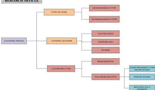
Figure 5 Clustering Process While designing a clustering algorithm, important parameters
that plays an important role are count, size and density of clusters. Based on number of parameters viz node types, algorithm type, control manner, cluster formation and CH selection, Network Architecture, etc. [10], a clustering algorithm is selected. Detailed clustering process is presented in Figure 5.
In WSN, a node can be considered as heterogeneous or homogeneous based on its capabilities. In case of homogeneous, all nodes have equal amount of energy and communication capabilities. This case leads to the decreased network lifetime as nodes that bypass most of the traffic will deplete their energy faster, this mostly happens with the nodes near the sink because whole network traffic bypass through them. Moreover transmission range, computational capabilities are other issues in homogeneous network case. So, load balancing is required in this case to improve network lifetime by distributing nodes in the network in an uneven manner. In LEACH [11], homogeneous nodes are considered and rotation of the CH is performed periodically to conserve energy. In [12], load balancing and energy efficiency are provided by incorporating gateways that calculate their distance to a sensor node through the IDs and location information broadcasted by sensor nodes. Minimum heap is used to balance the load in the network. Another example of homogeneous network is PEACH [13] protocol where selection of cluster head is done
from set of nodes and it aggregates the data and transmit it via single or multi-hop communication. Nodes in this protocol
have different transmission power levels and both location aware and location unaware protocols for WSNs are supported by this protocol. In heterogeneous case, some nodes are given more power in terms of energy, link and computation. Heterogeneity in WSN has been discussed in [14]. Heterogeneity is provided in terms of energy by choosing line powered nodes and link computation is provided by choosing backhaul links. Significant improvement of network in terms of lifetime and average delivery rate is observed. To enhance clustering, energy heterogeneity is discussed in [15] where modified clustering algorithm is proposed with three tier energy settings, where energy consumption among sensor nodes is adaptive to their energy levels.
distributed approach. Probabilistic or non-probabilistic algorithmic type defines a method of clustering process. Based on assigned probability to sensor nodes, CH is selected in probabilistic clustering method. In Highest Connectivity Cluster Algorithm (HCC)[17],based on highest connectivity of one hop neighbors, CH is selected and assigned with resources that has to be share among the members. Similar to HEED, a Distributed Weight-based Energy-efficient Hierarchical Clustering protocol (DWEHC)[18] is developed that uses different cluster sizes and that considers residual energy and location awareness in intra cluster topology.
To extend the sensor network lifetime, clustering is a key technique and incorporating load balancing in clustering will increase the lifetime of a sensor network by minimizing energy consumption. Scalability [19] can be increased by using load balancing in the network. A lot of algorithms exist in literature that used load balancing to improve network performance. In [19] heterogeneous network is considered, backup nodes are used to balance the load among clusters, efficient nodes are selected as cluster heads from the network and other nodes from the cluster that have high residual energy are considered as backup nodes. When CH reaches threshold value in terms of energy then backup nodes will replace the CH. This approach improves lifetime of the network. Load-balanced clustering has been discussed in [20] where clusters are formed with less energy constrained gateways acting as cluster head and load is balanced among them. Gateways are enabled with long haul communication capabilities. Based on the distance and communication cost, gateway calculates range set of sensors in its cluster and communicate this set with other gateways. Based on this information, two types of nodes are identified. Exclusive nodes that communicate only with one gateway and other nodes that communicate with other nodes. Load is balanced by minimizing the cost function which includes processing and communication load. Work discussed in [21] considers location information and connectivity density for establishing a more balanced clustering structure. Non-uniform distribution determines the cluster radiuses by evaluating the distance from the base station and connectivity density of nodes. Algorithm is compared with LEACH, HEED, and WBA. DSBCA minimizes energy consumption and improves the network lifetime with respect to other protocols.
Our work discusses new clustering approach that incorporates load balancing by assigning less number of nodes to CH's near the BS and by distributing number of nodes in a cluster in an efficient manner. Load Balancing (LB) technique reduces energy consumption, if LB is included in cluster based networks, it increases scalability. LB can apply in many ways viz. by using layered approaches, changing transmission level of CH and by varying cluster sizes. This paper propose an approach that perform load balancing in a network by varying cluster sizes in such a manner so that clusters near the sink are assigned with minimum number of nodes. CH's near the sink
are most heavily loaded nodes so load can be balanced by assigning less number of nodes. In this approach, distribution of nodes in a cluster in performed in an efficient manner. Number of nodes increases as we move away from the sink node but increment in node number has been performed by an order of one in a deterministic manner. In second phase of the paper, selection of ideal number of cluster head to be chosen for the given network has been discussed. Results are evaluated for different percentage of cluster heads and effectiveness of the approach has been evaluated by considering different network performance parameters. Section 3 discusses the energy consumption model used in the network followed by proposed approach. Simulation framework is presented in section 5 and effectiveness of the proposed approach is evaluated by the results.
3. SYSTEM MODEL 3.1.Radio Channel and Energy Dissipation
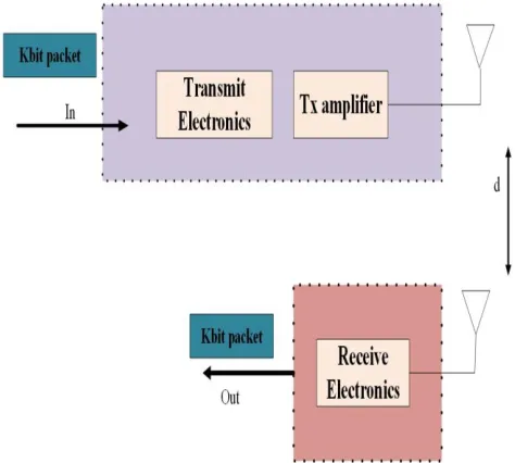
Energy model for sensor network is proposed by Heinzelman et. al [22]. This model includes basic energy dissipation of radio transmission that includes energy dissipated by transmitter and receiver electronics and includes micro-controller processing. But in sensor networks we cannot ignore processing energy as sensor networks involves processing both at sensor nodes and cluster head. Processing includes aggregating data, compute routing and maintain security etc. [23]. Energy is dissipated when sensor node is in idle mode, sleep mode and when it switches to either mode. When evaluating energy consumption of sensor nodes, these energy consumptions cannot be ignored. Energy consumption sources of a sensor node are micro controller processing, radio transceiver, transient energy while switching states, sensor sensing, sensor logging and actuation [24].
Basic energy consumption model based on [23] is shown in Figure 6 and Radio characteristics of classical model are presented in Table 1 that includes transmission, reception and idle mode. It does not include sleep and transition energy. This model includes transmitter and receiver electronics and energy dissipated while transmission and reception of a packet of k-bit over distance d. For transmission of a k bit packet, energy to be expanded is given by:
𝐸𝑡𝑛= 𝑒𝑒𝑙𝑒𝑐*k + 𝑒𝑎𝑚𝑝*k*𝑑𝑛 (1)
Where 𝑑𝑛 is power amplification factor and value of n varies for single hop and multi-hop communication. To receive a message of k bit, energy consumed by radio is given by:
𝐸𝑟= 𝑒𝑒𝑙𝑒𝑐*k (2)
Radio model Energy Consumption
Transmitter electronics 50nJ/bit
Receiver electronics 50nJ/bit
Transmission Amplifier 100pj/bit/𝑚2 Idle mode 40nJ/bit
Table 1 Radio Characteristics of Classical Model 3.2.Sensor Node energy computation
In this network, sensor node energy consumption involves sensing, transmitting and energy dissipated while in sleep and idle mode. Sensor node only senses the data and send it to CH in one hop communication. All processing takes place at cluster head. Different types of sensor nodes have different energy values for sensing, processing and radio hardware. Some examples of sensor motes are Mica, MicaZ, Telos B, Iris, WINS, Tiny Node, and Cricket. Mica Mote has sensing power of 0.015 W, processing power of 0.024 W, transmitting power of 0.036 W and reception power 0.02 W whereas WINS Mote has high power requirements as it has sensing power of 0.064 W, processing power of 0.360 W, transmission power of 3.75 W and reception power 1.87 W as provided by mannasim[25]. IRIS mote has higher transmission power and upto three times improved radio range than mica mote [26]. Comparing different energy consumptions, more energy is consumed in transmission as compared to processing and sensing. So, at transceiver, different power saving modes are enabled that includes sleep mode, idle mode and switching between these modes. Figure 7 represents state diagram of sensor node.
Sensing
Awake Transmis
sion
Idle radio Sleep
Sensor Node
inactive active inactive
active
Sensing state Sensed data
Other CH s inactive
Figure 7 State Diagram of Sensor Node
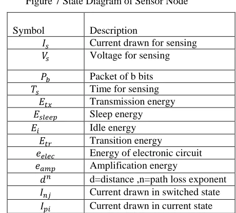
Table 2 Symbol Table for Sensor Energy Consumption Different symbols used here are presented in Table 2. Total energy consumption is the sum of Sensing energy (𝐸𝑠) and
Transceiver energy (𝐸𝑡).
𝐸𝑡𝑠=𝐸𝑠+𝐸𝑡 (3)
Sensing energy(𝐸𝑠) involves 𝐼𝑠 and 𝑉𝑠 that involves current and
voltage drawn while sensing activity and time 𝑇𝑠 is the total time duration for sensing a packet𝑃𝑏.
𝐸𝑠= 𝐼𝑠*𝑉𝑠*𝑃𝑏*𝑇𝑠 (4)
Transceiver energy includes transmission energy (𝐸𝑡𝑛), sleep
energy (𝐸𝑠𝑙𝑒𝑒𝑝), idle energy (𝐸𝑖) and energy consumed while
switching from sleep to idle mode (𝐸𝑡𝑟) and vice-versa.
Reception energy is not included in sensor node as only one Symbol Description
𝐼𝑠 Current drawn for sensing
𝑉𝑠 Voltage for sensing
𝑃𝑏 Packet of b bits
𝑇𝑠 Time for sensing
𝐸𝑡𝑥 Transmission energy
𝐸𝑠𝑙𝑒𝑒𝑝 Sleep energy
𝐸𝑖 Idle energy
𝐸𝑡𝑟 Transition energy
𝑒𝑒𝑙𝑒𝑐 Energy of electronic circuit
𝑒𝑎𝑚𝑝 Amplification energy
𝑑𝑛 d=distance ,n=path loss exponent
𝐼𝑛𝑗 Current drawn in switched state
hop communication is used and sensor nodes only transmit to respective cluster-heads.
𝐸𝑡= 𝐸𝑡𝑛 +𝐸𝑠𝑙𝑒𝑒𝑝 + 𝐸𝑖 + 𝐸𝑡𝑟 (5)
𝐸𝑡𝑛=𝑒𝑒𝑙𝑒𝑐*𝑃𝑏+ 𝑒𝑎𝑚𝑝*𝑃𝑏*𝑑𝑛 (6)
𝐸𝑠𝑙𝑒𝑒𝑝= 𝑉𝑠𝑙𝑒𝑒𝑝∗ 𝐼𝑠𝑙𝑒𝑒𝑝∗ 𝑇𝑠𝑙𝑒𝑒𝑝 (7)
𝐸𝑖= 𝑉𝑖∗ 𝐼𝑖∗ 𝑇𝑖 (8)
𝐸𝑡𝑟=
𝑉𝑡𝑟∗(𝐼𝑛𝑗− 𝐼𝑝𝑖)∗𝑇𝑡𝑟
2 (9)
So the total consumed energy at sensor node can be calculated by including sum of sensing energy, processing energy and transceiver energy.
𝐸𝑡𝑠=𝐼𝑠*𝑉𝑠*𝑃𝑏*𝑇𝑠 + 𝑒𝑒𝑙𝑒𝑐*𝑃𝑏+ 𝑒𝑎𝑚𝑝*𝑃𝑏*𝑑𝑛 + 𝑉𝑠𝑙𝑒𝑒𝑝∗
𝐼𝑠𝑙𝑒𝑒𝑝∗ 𝑇𝑠𝑙𝑒𝑒𝑝 + 𝑉𝑖∗ 𝐼𝑖∗ 𝑇𝑖 +
𝑉𝑡𝑟∗(𝐼𝑛𝑗− 𝐼𝑝𝑖)∗𝑇𝑡𝑟
2 (10)
3.3.Cluster head energy computation
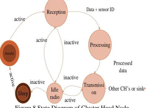
Cluster head receive data from sensor nodes, process the data and forward processed data to other CH's or sink. At CH, total energy consumption is sum of processing energy and transceiver energy. Cluster head start transmission when it receive data from sensor nodes, so it is kept in idle mode when it doesn't have any data to send. Various states of cluster head are presented in Figure 8.
Figure 8 State Diagram of Cluster Head Node Energy consumed at CH= Transmission energy (sink or other CH's) + Reception energy (sensor nodes within cluster + other CH's) + Processing energy.
𝐸𝑡𝑐=𝐸𝑝+𝐸𝑡 (11)
Transceiver energy (𝐸𝑡) includes reception energy (𝐸𝑟), transmission energy(𝐸𝑡𝑛), sleep energy (𝐸𝑠𝑙𝑒𝑒𝑝), idle energy (𝐸𝑖) and transition energy (𝐸𝑡𝑟).
𝐸𝑡= 𝐸𝑟+ 𝐸𝑡𝑛 +𝐸𝑠𝑙𝑒𝑒𝑝 + 𝐸𝑖 + 𝐸𝑡𝑟 (12)
CH receive data from sensor nodes(𝑆𝑗) and other CH's(𝐶ℎ𝑗)
while transmitting data to sink node. So the reception energy is sum of energy consumed while receiving data from sensor node and other CH’s. Transmission involves the energy consumed while transmitting data to sink via other CH’s. Multi-hop communication is used and in path loss exponent 𝑑𝑛, value of n is taken as 4.
𝐸𝑟= ∑𝑛𝑗=1𝑆𝑗(𝑒𝑒𝑙𝑒𝑐*𝑃𝑏) + ∑𝑛𝑗=1𝐶ℎ𝑗(𝑒𝑒𝑙𝑒𝑐*𝑃𝑏2) (13)
𝐸𝑡𝑛=∑𝑛𝑗=1𝐶ℎ𝑗(𝑒𝑒𝑙𝑒𝑐*𝑃𝑏2+𝑒𝑎𝑚𝑝*𝑃𝑏2* 𝑑𝑛 ) (14)
𝐸𝑠𝑙𝑒𝑒𝑝= 𝑉𝑠𝑙𝑒𝑒𝑝∗ 𝐼𝑠𝑙𝑒𝑒𝑝∗ 𝑇𝑠𝑙𝑒𝑒𝑝 (15)
𝐸𝑖= 𝑉𝑖∗ 𝐼𝑖∗ 𝑇𝑖 (16)
𝐸𝑡𝑟=
𝑉𝑡𝑟∗(𝐼𝑛𝑗− 𝐼𝑝𝑖)∗𝑇𝑡𝑟
2 (17)
Processing energy (𝐸𝑝):
𝐸𝑝= 𝑉𝑝∗ 𝐼𝑝∗ 𝑇𝑝 (18)
So total energy consumption as sum of processing and transceiver energy can be calculated as:
𝐸𝑡𝑠=𝑉𝑝∗ 𝐼𝑝∗ 𝑇𝑝 + ∑𝑛𝑗=1𝑆𝑗(𝑒𝑒𝑙𝑒𝑐*𝑃𝑏) + ∑𝑛𝑗=1𝐶ℎ𝑗(𝑒𝑒𝑙𝑒𝑐*𝑃𝑏2) +
∑𝑛𝑗=1𝐶ℎ𝑗(𝑒𝑒𝑙𝑒𝑐*𝑃𝑏2+𝑒𝑎𝑚𝑝*𝑃𝑏2* 𝑑𝑛 ) + 𝑉𝑠𝑙𝑒𝑒𝑝∗ 𝐼𝑠𝑙𝑒𝑒𝑝∗ 𝑇𝑠𝑙𝑒𝑒𝑝
+ 𝑉𝑖∗ 𝐼𝑖∗ 𝑇𝑖+
𝑉𝑡𝑟∗(𝐼𝑛𝑗− 𝐼𝑝𝑖)∗𝑇𝑡𝑟
2 (19)
Table 3. Symbol Table for Cluster Head Energy Consumption Different symbols used in Cluster Head energy consumption are presented in Table 3.
4. PROPOSED MODELLING
A new load balanced clustering approach is presented for network with different number of nodes. Variable cluster sizes are formed in the network, Clusters far from sink node has
Symbol Description
𝐸𝑡𝑐 Total CH energy
𝐸𝑟 Reception energy
∑ 𝑆𝑗
𝑛
𝑗=1
No. of sensor nodes that send data to CH.
∑ 𝐶ℎ𝑗
𝑛
𝑗=1
No. of parent CH's that send data to CH
𝑃𝑏2 Packet received from CH's
𝑃𝑏1 Packets received from catalyst
node Reception
Awake
Transmissi on Idle
radio Sleep
inactive
active
Other CH s or sink
Data + sensor ID
Processed data Processing
more number of nodes while clusters near sink node has very few nodes which prevents the problem of energy drainage of nodes near sink node. Earlier approaches presents arbitrary assignment of nodes in a cluster. In this approach precise assignment of nodes are presented in a cluster. This network is considered for stationary nodes. Following assumption are made:
I. Variable cluster sizes are chosen.
II. One hop communication between sensor nodes and CH and multi-hop communication between CH's takes place while transmitting data to sink node.
III. Network performance is evaluated for different number of CH's i.e. for 25% and 33% CH for whole network. IV. Network is analyzed for different number of nodes i.e. for
25,36,49,64 and 81 nodes.
V. Performance is evaluated for packet delivery ratio, average energy, throughput and delay.
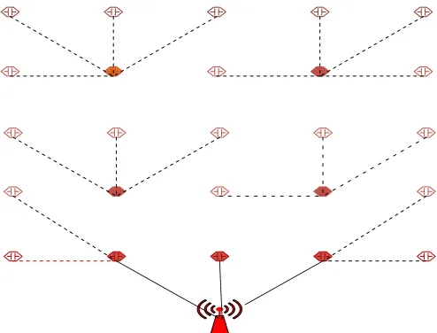
Proposed approach is presented in Figure 9. Variable cluster sizes are chosen and nodes in cluster decrease as we approach towards sink. A balanced clustering approach is used. CH's near sink are assign less number of nodes to avoid black hole problems near sink. This approach is extended for more number of nodes and is used in deterministic deployment only. Percentage of Cluster heads is varied across the network to find optimal number of CH's that enhance performance of the network in terms of different parameters. Grid topology is taken to evaluate the performance with Grid sizes of 5*5, 6*6, 7*7, 8*8, and 9*9. Objective of this work is to find the efficiency of deterministic network in terms of network lifetime, energy efficiency and other Quality of Service requirements. Using same given approach, network can be extended to more number of nodes.
Figure 9 Clustering Approach
5. RESULTS AND DISCUSSIONS 5.1.Simulator
Network simulator (ns-2) that is an open source, discrete event simulator for adhoc, wireless and wired, satellite networks has been used in this work to perform required simulations. Support for simulation of routing, multicast protocols and TCP over wired and wireless (local and satellite) networks [26] has been provided by ns-2. Ns-2 uses c++ and OTcl where c++ provides interface for developers to develop new protocols. This work is simulated on ns-2.35 on ubuntu-12.04 platform. 5.2.Performance Metrics
For evaluating performance of the network different metrics are used that includes Packet Delivery ratio (PDR), average energy, average throughput and average delay.
5.3.Simulation Parameters
Square grid topology is taken and results are examined for network consisting of 25,36,49,64 and 81 nodes. 25% and 33% of CH's are considered for simulation. AWK scripts and trace analyzer are used to evaluate results. By varying number of nodes and using AODV as routing protocol, network performance is analyzed. Different simulation parameters are shown in Table 4.
Parameter Value Number of nodes
MAC Radio Propagation Transmission Range
Initial Energy
25,36,49,64,81 MAC/802.11 Propagation/TwoRayGround
70 m 10 Table 4 Simulation Parameters 5.4. Effect on Packet Delivery Ratio
Ratio of number of packets received to number of packets sent defines Packet Delivery ratio (PDR). It is an important parameter to evaluate the network performance and higher PDR signifies better performance of the network. BS position has significant effect on PDR. Here in this network BS lies in lower central corner of the network.
84%. This shows significant performance in PDR compared to earlier approaches.
20 30 40 50 60 70 80 90
74 76 78 80 82 84 86 88 90
Packet Delivery ratio(packets/sec)
Number of nodes
25% CH 33% CH
Figure 10 No. of nodes v/s Packet Delivery Ratio 5.5.Effect on Average Energy
Energy consumption is the most important parameter for evaluating the performance of the network. If a node dies, a hole is created that will degrade the performance. To measure network performance, average energy values of all nodes in a network are taken. Average energy is the measure of total energy left divided by total number of nodes. Initially 10 joules of energy is taken. Minimum amount of energy is taken to evaluate network performance in case where continuous data is sent and amount of energy withdrawn will be more.
Figure 11 Number of nodes v/s Average energy
Figure 11 represents energy vs. number of nodes. It is observed average energy is more in case of 33% CH. This is due to fact that with more number of CH’s, transmission energy will be reduced as CH’s do not transmit over long distances as in case of 25% CH. Transmission energy is the major source of energy consumption so results are found better when more number of CH’s are involved.
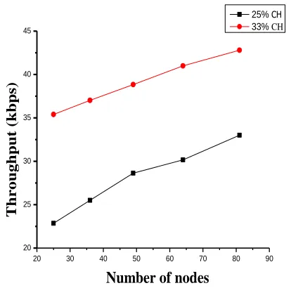
5.6.Effect on throughput
Throughput determines efficiency and is defined as a rate at which a source receives data packets per unit time in a network. It is measured in bits per second (bit/s) [27].
Throughput = 𝑁𝑢𝑚𝑏𝑒𝑟 𝑜𝑓 𝑝𝑎𝑐𝑘𝑒𝑡𝑠 𝑟𝑒𝑐𝑖𝑒𝑣𝑒𝑑𝑁𝑒𝑡𝑤𝑜𝑟𝑘 𝑜𝑝𝑒𝑟𝑎𝑡𝑖𝑜𝑛 𝑡𝑖𝑚𝑒 [28] (21) Throughput should be higher for better network performance. From Figure 12, it is observed that more efficiency in throughput is observed for 33% CH as compared to 25% CH. Average value of throughput is taken to evaluate the results.
20 30 40 50 60 70 80 90
20 25 30 35 40 45
Thro
ughpu
t (k
bp
s)
Number of nodes
25% CH
33% CH
Figure 12 Number of nodes v/s Average Throughput 5.7.Effect on average delay
Average delay is calculated by taking average value of end to end delay where end to end delay is the time a packet taken by a packet while travelling from source to destination.
End to end delay = 𝑇𝑑 - 𝑇𝑠
Where 𝑇𝑑 is reception time of packet at destination and 𝑇𝑠 is
20 30 40 50 60 70 80 90 0.6
0.8 1.0 1.2 1.4 1.6 1.8 2.0 2.2 2.4
Dela
y
Number of nodes
25 % CH
33% CH
Figure 13. Number of Nodes v/s Delay
It is analyzed from simulation results [Table 5] that ideal range of cluster heads can be found between 25-33%. If we take packet delivery ratio as a performance metric, more efficient results are achieved with more number of cluster heads. Average delay is found more in case of 25% cluster heads. With 33% of cluster heads, throughput and PDR is maximized and energy savings increases. The results are achieved due to increased number of cluster heads and energy is also effected as more number of cluster heads leads to less number of nodes assigned to cluster heads near the sink. Load is balanced and more nodes that act as cluster heads participate in data forwarding which leads to high PRR and less energy consumption. Assigning less number of nodes near sink increases network lifetime. This approach when implemented with more number of CH provides efficient results for QoS based applications.
NODES PDR% 25%
PDR% 33%
AVG ENERGY 25%
AVG ENERGY 33%
THROUGHPUT (kbps) 25%
THROUGHPUT (kbps) 33%
AVERAGE DELAY(sec) 25%
AVERAGE DELAY(sec) 33% 25 83 90 3.28 3.64 22.86 35.39 0.96 .70
36 80.6 87 3.02 3.25 25.51 37.01 0.98 0.75
49 78 85.3 2.24 2.54 28.63 38.84 1.12 0.94 64 75.5 81.4 0.59 0.98 30.16 41 1.65 1.41
81 74 80 0.27 1.25 33.0 42.8 2.32 1.93
Table 5 Simulation Results 6. CONCLUSION
Topology, cluster distribution, cluster count plays important role in network performance. Square grid topology is taken and new clustering approach with load distribution is implemented. Results with different number of nodes i.e. 25, 36,49,64,81 are analyzed for 25% and 33% CH's. From results, it is concluded that higher packet delivery ratio, average energy and throughput is observed for 33% CH's and high average delay is observed for 25% CH. So, better network performance can be achieved with 33% CH's in the network if network demands reliability as reliability is linked with high packet reception ratio. Depending upon the application to be used, ideal number of nodes acting as cluster head can be found.
REFERENCES
[1] G. Tuna, R. Das, A. Tuna, “Wireless Sensor Network-Based Health Monitoring System for the Elderly and Disabled”, International Journal
of Computer Networks and Applications (IJCNA), Volume 2, Issue 6, November – December (2015), pp. 247-253.
[2] R.K.Jha,A.Singh,A.Tiwari,P.Shrivastava,”Performance Analysis of Disaster Management using WSN Technology”,Procedia Computer Science ,2015, pp.162-169.
[3] D. Chen and P. K. Varshney, “QoS Support in Wireless Sensor Network: A Survey,” Proceedings of the International Conference on Wireless Networks (ICWN 04), Las Vegas,June 2004, pp. 227-233.
[5] Las Vegas, Nevada, Las Vegas, Nevada, Mohamed Younis, Kemal Akkaya, “Strategies and techniques for node placement in wireless sensor networks: A survey”, Ad Hoc Networks, vol. 6, 2008, pp. 621–655. [6] Akhilesh Shrestha and Liudong Xing, "A performance comparison of
Different topologies for wireless sensor networks",IEEE Conference on Technologies for Homeland Security,2007, pp. 280-285.
[7] Wint Yi Poe,Jens B. Schmitt,"Node deployment in large Wireless Semsor Networks:Coverage,Energy Consumption and Worst-Case Delay", AINTEC '09 Asian Internet Engineering Conference ,2009, pp.77-84. [8] Quazi Mamun, " A Qualistative Comparison of Different Logical
Topologies for Wireless Sensor Networks",SENSORS, , vol. 12, 14887-14913. 2012.
[9] Liudong Xing and A. Shrestha, " QoS Reliability of Hierarchial Clustered Wireless Sensor Networks", In Proceedings of 25th IEEE International Conference on Performance,Computing and Communications,April 10-12,2006.
[10] Sukhkirandeep Kaur,Roohie Naaz Mir,"Clustering in Wireless Sensor Networks-A Survey",I.J. Computer Network and Information Security ,vol. 6,2016, pp.38-51.
[11] W.Heinzelman, A.Chandrakasan, and H. Balakrishnan,“Energy-Efficient Communication Protocols for Wireless Microsensor Networks”, Proceedings of the 33rd Hawaaian International Conference on Systems Science (HICSS), January 2000.
[12] P. Kuila, P. K. Jana, “Energy Efficient Load-Balanced Clustering Algorithm for Wireless Sensor Networks”, 2nd International Conference on Communication, Computing & Security [ICCCS-2012],2012, pp-771-777,.
[13] Xuxun Liu, “A Survey on Clustering Routing Protocols in Wireless Sensor Networks”, Sensors, vol. 12,Aug. 2012, , pp. 11113–11153. [14] Mark Yarvis, Nandakishore Kushalnagar, Harkirat Singh, " Exploiting
Heterogeneity in Sensor Networks"Proceedings IEEE 24th Annual Joint Conference of the IEEE Computer and Communications Societies.,vol. 2, 2005,pp. 878-890.
[15] Femi A. Aderohunmu, Jeremiah D. Deng, Martin Purvis, " Enhancing Clustering in Wireless Sensor Networks with Energy Heterogeneity", 18 International Journal of Business Data Communication and Networking",vol.7,no.4,2011,pp. 18-31.
[16] R.M.B. Hani and A.A. Ijjeh, “A survey on leach based energy aware protocols for wireless sensor networks”, Journal of communication, vol. 8, 2013.
[17] S. Banerjee and S. Khuller, “A clustering scheme for hierarchical control in multi-hop wireless networks”, in Proceedings of 20th Joint Conference of the IEEE Computer and Communications Societies (INFOCOMŠ 01), Anchorage, AK, April 2001.
[18] R. Tandon, B. Dey and S. Nandi, “Weight based clustering in wireless sensor networks”, Communications (NCC), 2013.
[19] Dipak Wajgi1 and Dr. Nileshsingh V. Thakur2," LOAD BALANCING BASED APPROACH TO IMPROVE LIFETIME OF WIRELESS SENSOR NETWORK, International Journal of Wireless & Mobile Networks (IJWMN), vol. 4, No. 4, August 2012.
[20] Gaurav Gupta, Mohamed Younis, “Load-Balanced Clustering of Wireless Sensor Networks",in Proc. IEEE International Conference on Communications(ICC’03),vol. 3,May 2003,pp.1848-1852.
[21] Ying Liao, Huan Qi, and Weiqun Li,"Load-Balanced Clustering Algorithm With Distributed Self-Organization for Wireless Sensor Networks", IEEE SENSORS journal, vol. 13, no. 5, May 2013. [22] N. Kamyabpour, D.B. Hoang, “Modeling overall energy consumption in
wireless sensor networks”, 11th International Conference on Parallel and Distributed Computing, Applications and Technologies, PDCAT-10, December 2010, pp. 8–11
[23] M. N. Halgamuge, M. Zukerman, K. Ramamohanarao, and H. L. Vu, "An estimation of sensor energy consumption," Progress In Electromagnetics Research B, vol. 12, 259-295, 2009.
[24] Rodolfo Miranda Pereira, Linnyer Beatrys Ruiz, Maria Luisa Amarante Ghizoni," MannaSim: A NS-2 extension to simulate Wireless Sensor Network",ICN: The Fourteenth International Conference on Networks,2015.
[25] http://www.isi.edu/nsnam/ns/
[26] Norashidah Md Din, M.Z. Jamaludin,"Trace Analyzer for NS-2",IEEE,2006
[27] Mridula Maurya, Shri R.N. Shukla," Current Wireless Sensor Nodes(Motes):Performance metrics and constraints",International Journal of advanced research in Electronics and Communication Engineering(IJARECE),volume 2, Issue 1, January 2013.
[28] M. Kavitha, B. Ramakrishnan, Resul Das, “A Novel Routing Scheme to Avoid Link Error and Packet Dropping in Wireless Sensor Networks”, International Journal of Computer Networks and Applications (IJCNA), volume 3, Issue 4, July – August, 2016, PP. 86-94, DOI: 10.22247/ijcna/2016/v3/i4/48569.
Authors
Sukhkirandeep Kaur is a research scholar in the Department of Computer Science & Engineering at NIT Srinagar, INDIA. She received her B.Tech in Computer Science & Engineering from Punjabi University, Patiala(India) in 2010 and M.Tech in Computer Science & Engineering from Lovely Professional University, Jalandhar(India) in 2012. Her research interests include Routing and Clustering in Wireless Sensor Networks.