Computational Modelling of HT Carcinoma Cells using different Averaging Tree Techniques

International Journal of Advanced Trends in

Computer Applications

www.ijatca.com

Computational Modelling of HT Carcinoma

Cells using different Averaging Tree Techniques

1

Shruti Jain, 2D S Chauhan

1

Department of Electronics and Communication Engineering, Jaypee University of Information Technology, Solan, HP. 173234, India.

2

GLA Mathura, Uttar Pradesh, 281406, India

1

[email protected]

Abstract:

Keywords:

I.

INTRODUCTION

Data mining methods can be helpful in identifying covariates related to adverse events. Predictive modeling and data mining have the potential to identify groups at high risk. The regulatory impact of predictive modeling is not clear at this time. A huge amount of web searches are daily created through search engines.

Social media and communities have become

increasingly important data. The health industry and medical field generate bytes of data from patient monitoring, medical record and medical imaging. Global telecommunication networks create tremendous data traffic every day. This triggered the idea of combining benefits and advantages of reality mining, machine learning and Big Data predictive analytics tools, applied to sensors real time. The development of effective predictive and perspective analytics systems relies on the use of advanced and preformed technologies such as Big Data, advanced analytics tools and intelligent systems.

In this paper, we are working with marker proteins [1-3] which occur due to the combination of TNF [4-5], EGF [6-8] and insulin [9-11]. In general, there are two

types of data consisting of continuous and categorical. For the categorical method, we usually use machine learning algorithms while for continuous data, classification trees / Single regression trees and Averaging Trees/ decision trees method is considered. Logistic regression (LoR) is one which is applied for continuous and categorical data both. It usually uses

maximum likelihood estimation (MLE) after

transforming the dependent variable into a log it variable and gives a better result for large data set in spite of small data sets. This type of regression neither requires normally distributed variables nor does it assume a linear relationship between the dependent and independent variables.

survival/ death. In boosting tree, the division is on the basis of ten different concentrations of TNF, EGF, and Insulin while in RF method, the model is made for the training and testing of data on the basis of samples.

The organization of the paper is as: Section 2 explains the dataset used for the simulations and explains the proposed model, Section 3 explains the experimental and simulation results of the proposed model which is followed by the conclusion and future work.

II.

MATERIALS AND METHODS

There are various steps for processing the data which helps in extracting the results from input data/ images:

2.1 Materials:

The data was collected from the heat map taken from [3] for the HT carcinoma cells which help in cell survival/ death. In this paper we have considered the three input proteins (TNF, EGF and Insulin) and four different outputs which results in different proteins consisting ptAkT, IKK, MK2, AkT, JNK, MEK, ERK, IRS, FKHR, pAkT, and EGFR. We can also say that if these proteins are absent or electronically zero (0) then it leads to cell death but if these proteins are present or electronically one (1) then there is cell survival. We have collected the data for all marker proteins for ten different concentrations of input proteins (in ng/ml). All the simulations were carried out in Statistical and SPSS software.

2.2 Proposed Methodology:

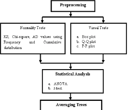
This paper proposes a model using different averaging tree techniques that help in diagnosis of cell survival/ death for HT carcinoma cells using three different inputs with ten different combinations. Fig 1 explains the steps followed for the proposed model.

2.2.1 Data Pre-processing:

In pre-processing main steps consisting data

integration, data reduction, data cleaning, data discretization, and data transformation.

1.Data cleaning involves the identifying or removal of outliers, smoothening of noisy data, or filling the missing values, etc. Noisy data can be solved by different ways consisting of binning

methods, clustering and regression. In clustering;

we can detect and remove outliers while for

Regression; smoothening of data is done by fitting

into regression function. Binning method consists

of two types of partitioning: equal depth/

frequency partitioning where the range is divided

into N intervals with the same number of samples.

Through this method, we obtain good data scaling. Categorical attributes managing is a little bit tricky in this partitioning. This type of partitioning does

not handle skewed data. Second is Equal

width/distance partitioning where the range is

divided into N equal size intervals. If we have A

and B as the lowest and highest value of feature

than the width of the interval is expressed by Eq. (1)

W = (B-A) / N (1)

2.Data Integration:

This includes removing redundant or duplicates data. Detecting and resolving data which involve conflicts. Chi-square test is done for calculating correlation or covariance values. If the data is is continuous than regression analysis is performed and if it is categorical than chi-square test is applied.

3.Data Transformation:

This step involves normalization, smoothening and aggregation of data. Normalization is of different

types consisting min-max approach,

numerosity reduction, data cube aggregation, and

dimensionality reduction. In dimensionality

reduction, there are two step feature selection and heuristic methods. Feature selection is of two types first is direct method in which selection of a minimum set of feature (attribute) is done which is sufficient for data mining while second is indirect method consists of principal component analysis (PCA), singular value decomposition (SVD), independent component analysis (ICA). The heuristic method involves stepwise forward selection, backward elimination and both.

5.Data Discretization:

In this type division of range for the continuous features was done into intervals because some data

mining algorithms only accept categorical

attributes. This can be done by binning method or entropy-based method. The discretization of numeric/ categorical data can be done by binning method, histogram analysis or clustering analysis.

2.2.2 Feature Selection and Feature extraction:

After pre-processing, feature extraction is applied using any of the technique consisting of Morphological and Texture [15-17]. Morphological methods help in calculating the shape based properties. Texture Method (TM ) is subdivided into three sub different methods as Signal Processing (SP) which calculates law mask features, Transform Domain (TD) calculates wavelet packet transform (WPT), FPS and Gabor Wavelet transform (GWT), and Statistical feature (SF) calculates different gray level matrixes [18-19].

2.2.3 Data Partitioning:

For validation of data it is divided into two parts one is known as testing while another is known as training. Data partitioning is done by different methods as hold out, stratified sampling, boot-strap, resampling or three-way data splits. In general hold out approach is used in which we can divide the dataset into ⅔ to the

⅓ ratio where ⅔ for training and ⅓ for testing. Hold out can be single hold out or repeated holdout. Cross-validation (CV) can also be done by using k- fold CV

or leave one out CV. Fork- fold CV, we can train k-1

partitioned data while rest dataset is used for testing. In

leave one out CV we can train k = n data.

2.2.4 Data Classification:

There are different algorithms through which we can classify the data. Basically, we have three algorithms consisting of Classification trees / Single regression trees, Averaging Trees/ Decision Trees and Machine learning algorithms. The Classification trees / Single regression trees are subdivided as Classification and Regression Trees (CRT models, CART, CHI),

Interactive C&RT algorithm (ICR), Interactive

Exhaustive CHAID algorithm (IEC)and Chi-squared and Interactive Decision (CHAID). The Averaging Trees/ Decision Trees consisting Bagging Trees (BT) known as Averaging Trees, Random Forests (RF) known as Cleverer Averaging of Trees and Boosting Trees (BOT) known as Cleverest Averaging of Trees. The different Machine learning algorithms are kNN, Artificial Neural Networks (ANN) [18] and Support Vector Machines (SVM) [19].

III.

RESULTS AND DISCUSSIONS

Figure 2: Different static summary, box plot and P-P plot

Table 1: Normality tests using KS, AD, and Chi-square

K-S d K-S AD Stat AD p-value

Chi-sq Chi-sq p-value

Chi-sq df Gaussian Mixture 0.03 0.98 0.15 1.00 6.07 0.11 3

Normal (location, scale) 0.18 0.00 18.50 0.00 193.53 0.00 7

Log Normal (scale, shape) 0.21 0.00 25.51 0.00 232.73 0.00 6

Half Normal (scale) 0.23 0.00 22.62 0.00 266.73 0.00 7

Rayleigh (scale) 0.24 0.00 23.26 0.00 279.47 0.00 7

Weibull (scale, shape) 0.57 0.00 117.27 0.00 1424.27 0.00 8

General Pareto (scale,

shape) 0.64 0.00 144.16 0.00 1907.27 0.00 8

Triangular(min, max,

mode) 0.87 0.00 532.70 0.00 1555.27 0.00 7

A statistical test is applied to get the best proteins which detect cell survival/ death. Out of eleven proteins, seven proteins (AkT, MK2, JNK, ERK, EGFR, IRS and FKHR) found the better for further analysis.

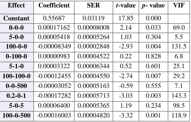
Table 2: Regression analysis in terms of standard error coefficients, p-value, t-value and VIF for FKHR

Effect Coefficient SER t-value p- value VIF Constant 0.55687 0.03119 17.85 0.000

0-0-0 0.00017162 0.00008008 2.14 0.033 69.0 Summary: FKHR

K-S d=.23157, p<.01 ; Lilliefors p<.01 Expected Normal

0.45 0.46 0.47 0.48 0.49 0.50 0.51 0.52 0.53 0.54 X <= Category Boundary

0 10 20 30 40 50 60 70 80 90 100 110 N o . o f o b s.

Mean = 0.5057 Mean±SD = (0.4848, 0.5266) Mean±1.96*SD = (0.4647, 0.5467) 0.46 0.47 0.48 0.49 0.50 0.51 0.52 0.53 0.54 0.55 F K H R

Normal P-Plot: FKHR

0.46 0.47 0.48 0.49 0.50 0.51 0.52 0.53 0.54 Value -4 -3 -2 -1 0 1 2 3 4 E xp e ct e d N o rm a l V a lu e Summary Statistics:FKHR Valid N=300

% Valid obs.=100.000000 Mean= 0.505715

Confidence -95.000%= 0.503340 Confidence 95.000%= 0.508090 Geometric Mean= 0.505277 Harmonic Mean= 0.504831 Median= 0.515829 Mode=Multiple

Frequency of Mode= 1.000000 Sum=151.714454

Minimum= 0.464025 Maximum= 0.535192 Variance= 0.000437 Std.Dev.= 0.020906

Confidence SD -95.000%= 0.019356

Standard Error Coefficients (SER) is used to measure precision. The smaller the value the more precise is the estimate. If SER is divided by coefficient values, than

we obtain the t-value. Table 2 shows the Standard

Error Coefficient (SER), t-value, p-value and variance

inflation factor (VIF) for FKHR.

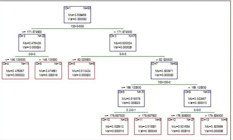
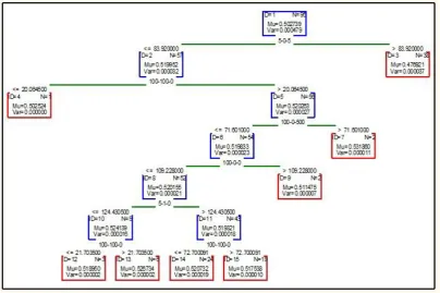
Lastly, different approaches of averaging/decision trees are applied to get which protein helps in cell survival/ death. In the paper, we are using boosted trees and

random forest for modeling our system. In Boosted

trees, we compute a sequence of simple trees, where

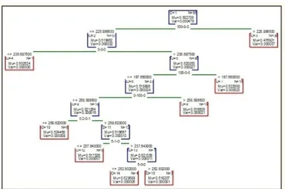
each successive tree is built for the prediction residuals of the preceding tree. This method is used to build binary trees, means the partition of the data into two samples at each split node. Fig 3 shows the boosted trees of AkT for 6 nonterminal and 7 terminal nodes, Fig 4 to Fig 6 shows the boosted trees of ERK, JNK, and MK2 respectively for 7 nonterminal and 8 terminal nodes. Fig 7 and Fig 8 shows the boosted trees of EGFR, and IRS respectively for 7 nonterminal and 8

terminal nodes. Each figure is showing the mu and var

value of each division.

Figure 3: Boosted tree graph for AkT

Figure 7: Boosted tree graph for EGFR

Figure 8: Boosted tree graph for IRS

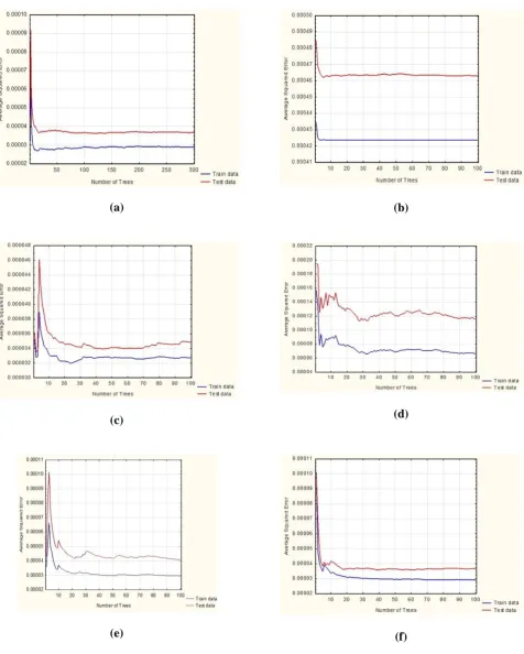
Random Forest (RF) is a refinement of bagging tree

method. In the RF method, m feature was extracted if

we have p number of total features or we can say m

=√p or log2p. RF method improves the bagging tree by

de-correlating the trees and have the same expectation.

(a) (b)

(c) (d)

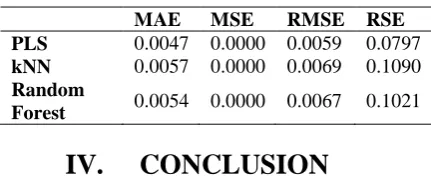
Table 3: Various error function for FKHR

MAE MSE RMSE RSE

PLS 0.0047 0.0000 0.0059 0.0797 kNN 0.0057 0.0000 0.0069 0.1090 Random

Forest 0.0054 0.0000 0.0067 0.1021

IV.

CONCLUSION

This paper presents the proposed model for cell survival/ death by using Random forest and boosting tree and random forest methods which are different Averaging tree techniques. The data is collected which is pre-processed by normality test and visual plots. The marker proteins were selected from eleven different proteins by using statistical analysis. Lastly, averaging tree technique is applied to the data set to predict which protein or sample helps in cell survival/ death. In boosting tree, the division is on the basis of ten different concentrations of TNF, EGF, and Insulin while in RF method, the model is made for the training and testing of data on the basis of samples. 100-0-500 ng/ml yields the better results using boosting tree and from RF methods we come across that FKHR protein leads to cell death while rest proteins help in cell survival if they are present. In the future, deep learning algorithms can be applied on the dataset.

References

[1] S Jain., Communication of signals and responses leading to cell survival / cell death using Engineered Regulatory Networks. PhD Dissertation, Jaypee University of Information Technology, Solan, Himachal Pradesh, India, 2012.

[2] R Weiss., Cellular computation and communications using engineered genetic regulatory networks. PhD Dissertation, MIT, 2001.

[3] S Gaudet, JA Kevin, AG John, PA Emily, LA Douglas, and SK Peter. A compendium of signals and responses triggered by prodeath and prosurvival cytokines. Manuscript M500158-MCP200, 2005.

[4] S Jain, PK Naik, R Sharma, A Computational Modeling of cell survival/ death using VHDL and MATLAB Simulator, Digest Journal of Nanomaterials and Biostructures. 2009: 4 (4): 863- 79.

[5] JA Kevin, AG John, G Suzanne, SK Peter, LA Douglas, YB Michael. A systems model of signaling identifies a molecular basis set for cytokine-induced apoptosis. Science. 2005; 310, 1646-53.

[6] N Normanno, A De Luca, C Bianco, L Strizzi, M Mancino, MR Maiello, A Carotenuto, G De Feo, F Caponiqro and DS Salomon. Epidermal growth factor receptor (EGFR) signaling. Cancer Gene. 2006; 366, 2-16. [7] S Jain, Implementation of Marker Proteins Using Standardised Effect, Journal of Global Pharma Technology. 2017: 9(5), 22-27.

[8] S Jain, Compedium model using frequency / cumulative distribution function for receptors of survival proteins: Epidermal growth factor and insulin, Network Biology. 2016: 6(4), 101-110.

[9] S Jain, PK Naik and SV Bhooshan. Mathematical modeling deciphering balance between cell survival and cell death using insulin. Network Biology. 2011; 1(1):46-58. [10] JM Lizcano and DR Alessi. The insulin signalling pathway. Curr Biol.2002; 12, 236-38.

[11] MF White. Insulin Signaling in Health and Disease. Science. 2003; 302, 1710–11.

[12] S Jain, Parametric and Non Parametric Distribution Analysis of AkT for Cell Survival/Death, International Journal of Artificial Intelligence and Soft Computing. 2017 : 6(1), 43- 55

[13] A. Brunet, A. Bonni, M. J. Zigmond, M. Z. Lin, P. Juo, L. S. Hu, Akt promotes cell survival by phosphorylating and inhibiting a Forkhead transcription factor. Cell, 96 (1999), 857–868.

[14] S Jain, Regression analysis on different mitogenic pathways, Network Biology. June 2016: 6(2), 40-46 . [15] S. Bhusri, S. Jain, and J Virmani, Classification of Breast Lesions Using the Difference of Statistical Features, Research Journal of Pharmaceutical, Biological and Chemical Sciences(RJPBCS), july-aug 2016,pp. 1366. [16] S.K. Alam, E.J. Feleppa, M.Rondeau, A. Kalisz, and B.S. Garra,Ultrasonic multi-feature analysis procedure for computer-aided diagnosis of solid breast lesions,2011. vol. 33, no. 1, pp. 17–38.

[17] S. Rana, S. Jain, and J. Virmani, SVM-Based characterization of focal kidney lesions from B-Mode ultrasound images, research J of pharmaceutical, biological and chemical sciences (RJPBCS). July-Aug 2016,vol. 7(4), pp.837.

[18] A.Dhiman, A. Singh, S.Dubey and S. Jain, Design of lead II ECG Waveform and Classification performance for Morphological features using Differenct Classifiers on lead II, Research J of pharmaceutical, biological and chemical sciences, July-Aug 2016, pp. 1226-1231.