MAGNETIC ORDERING PHENOMENA
IN THE HEXAGONAL ABX3 HALIDES,
A
NEUTRON SCATTERING STUDY
by
Andrew Ross Monteith
A doctoral thesis submitted in the partial fulfilment of the requirements
for the award of Doctor of Philosophy
at University College London
ProQuest Number: U642237
All rights reserved
INFORMATION TO ALL USERS
The quality of this reproduction is dependent upon the quality of the copy submitted.
In the unlikely event that the author did not send a complete manuscript and there are missing pages, these will be noted. Also, if material had to be removed,
a note will indicate the deletion.
uest.
ProQuest U642237
Published by ProQuest LLC(2015). Copyright of the Dissertation is held by the Author.
All rights reserved.
This work is protected against unauthorized copying under Title 17, United States Code. Microform Edition © ProQuest LLC.
ProQuest LLC
789 East Eisenhower Parkway P.O. Box 1346
Index
Abstract 5
List of Figures 6
List of Tables 11
Acknowledgements 12
1 Introduction 15
2 Theory 24
2.1 Second Order Phase Transitions. 24
2.2 Heisenberg Triangular Antiferromagnets 32
2.2.7 Easy A xis A nisotropy: D < 0 33
2.2.1.1 The H aldane conjecture. 36
2.2.2 Easy Plane A nisotropy, D > 0 4 0
2.2.2.1 L arge E asy Plane A n isotropy 4 0
2.2.2.2 Sm all E asy Plane A nisotropy 42
2.2.3 D istorted L attice 43
2.3 Singlet Ground State Antiferromagnets 47
2.3.1 True sin glet ground state antiferrom agnets, (CsFeBrs, CsFeClj). 4 8 2.3.2 Induced m om ent antiferrom agnets, (RbFeBr3, RbFeCls). 49
2.4 Neutrons: their properties and applications. 52
2.4.1 Fundam ental p ro p erties o f the neutron. 52
2.4.2 Production o f neutrons. 53
2.4.3 Diffraction. 56
2.4.3.1 E lastic scattering 56
2.4.3.2 Inelastic scattering 63
2 .4.3.3 M agnetic Scattering 65
3 Experimental Methods 69
3.1 Crystal Growth M ethods 69
3.2 The Neutron Scattering Spectrometers/Diffractometers. 71
3.2.1 Triple A xis S pectrom eter 71
3.2.1.1 The TAS E l a t the HMl, Berlin. 76
3.27.2 The TAS V2 (FLEX) a t the HMI, Berlin. 77
3.2.7.3 The TAS 4F1 an d 4F2 a t the LLB, Saclay, Paris. 78 3.2.7.4 The Single C rystal Diffractometer, D 15 a t the ILL, G renoble. 79 3 .2 7 .5 The M em brane Diffractometer, VI a t the HMI, Berlin. 80
3.2.2 P ow der D iffractom eter. 81
3.2.2.1 The P o w d e r Diffractometer, HRPD, a t the ISIS fa cility, Oxford. 85 3.2.2.2 The P o w d e r Diffractometer, POLARIS, a t the ISIS fa cility, Oxford. 8 7
3.2.3 F lat Cone D iffractom eter. 89
3 .2 .3 .1 The F lat Cone Diffractometer, E2 a t the HMI, Berlin. 91
3.3 Sample Environment 93
3.3.7 The ILL O range Cryostat. 93
3.3.2 Dilution Refrigeration Units 94
3.3.3 G as/Liquid Pressure Cells. 96
3.3.4 H orizontal an d Vertical M agnets 98
3 .3 .4 .1 The Vertical M agnet, VM3, a t the HMI, Berlin. 98
Index
4 Chiral Order in ABX3 compounds 101
4.1 CsMnBraCEl, V I - H M I ) 101
4.1.1 Tem perature D ependence o f the M agnetic O rdering in CsMnBr^ in the presen ce o f an
E lectric Field. 108
4.1.2 E lastic Scattering on CsM nBrj in the presen ce o f an E lectric f ie ld a n d a M agn etic field. 114
4.2 C sNiCls (E 1 / E2 - HMI) 119
4.2.1 E lastic Scattering on CsN iC lj in the p resen ce o f a m agnetic field . 120 4.2.2 Diffuse M agnetic Scattering fro m CsNiCls around the transition point. 127
4.3 RbNiCla (4F1) 132
4.3.1 E lastic Scattering on RbNiCls under the Presence o f H ydrostatic Pressure. 133
4.4 TlFeCla 136
4.4.1 Structural C haracterisation o f TlFeCl3. 137
4.4.2 M agn etic C haracterisation o f TlFeCls. 142
4.5 KNiClj (4F2 - LLB) 147
4.5.1 M ixed Phase 147
4 .5 .2 Azl X 4di X c ph ase 152
4.5.3 R T p h ase 156
5 Singlet Ground State AFeXs compounds 162
5.1 C sFeCl] (LLB) 162
5 .1.1 M agnon dispersion m easurem ents on CsFeCls under h ydrostatic pressure. 162 5.1.2 Structural studies on CsFeCls under h ydrostatic pressure. (ISIS) 167
5.2 CsFeBfa (LLB) 173
5.2.1 M agnon dispersion m easurem ents on CsFeBrs under h ydrostatic pressure. 173 5.2.2 Structural studies on CsFeBrs under h ydrostatic pressure. 177
5.3 CsFeBrs (V 2) 180
5.3.1 E lastic Scattering. 181
5.3.2 Inelastic Scattering. 186
6 Conclusions, Outlook 197
Abstract _________________________________________________________________
Abstract
M ost ABX3 materials (where A is a lA group cation, B is a divalent first row
transition metal cation and X is a halide ion) possess a hexagonal perovskite structure
where chains o f face sharing BXô octahedra align along the c - axis separated by the
A ions. This results in an interchdin separation that is much larger than the intrachain
separation leading to a quasi one-dimensional magnetic behaviour at low temperature.
The magnetic character of the compounds is strongly dependent on the nature and
strength o f the superexchange pathways and the environment around the B^ ion,
manipulation of which leads to new and interesting physics. The structural properties
of the ABX3 materials allow them to be used as model systems for a variety of
conjectures. The chain like structure allows compounds such as CsNiCl3 and RbNiCl3
to be used as model systems for the Haldane conjecture, whilst the triangular
arrangement of the spins on the B^^ ions allows compounds such as CsMnBr3 to be
used as model systems for the Chiral Universality class conjecture o f Kawamura.
This thesis is concerned with the investigation of the crystallographic and magnetic
properties o f some the ABX3 family of compounds by means of neutron scattering;
specifically to observe the effects of extreme sample environment on the systems,
such as applied hydrostatic pressure, applied magnetic and electric field etc.
Magnetostructural correlations have been made for CsFeC^ and CsFeBr3 on the basis
of inelastic and powder neutron diffraction studies on the systems under pressure.
Characterisation of the p and y-phase of KNiCb have been performed using inelastic
neutron diffraction measurements and the magnetic and structural phase diagrams of
TlFeCh have also been mapped out. The magnetic phase diagram o f CsNiCl3 has
been studied and a proof of the existence o f a magnetoelectric effect in CsMnBr3 has
List of Figures
List of Figures
Figure 1: The magnetic dispersion curves for (a) the S=3/2 chain compound CsVClj and (b) the
S=l/2 chain compound KCuFj. 16
Figure 2; Structure of the Lai xSr^MnO], Lai.xSrxMn0 4 and Lai xSrxMnzO? compounds". 17
Figure 3: Basic structure of the triangular, kagome and tetragonal arrays. 17
Figure 4: Simplified schematic of the phase diagram for the Ising - Heisenberg chain. 21
Figure 5: Ground state spin configuration of 3 Ising spins on a triangle. Frustration leads to a
non trivial degeneracy of the ground state. 28
Figure 6: The twofold degenerate ground state for an XY antiferromagnet on a triangular lattice,
showing the two different chiral states (a) and (b). 28
Figure 7: Chiral degeneracy in the ordered state of the XY antiferromagnet, (a) and the XY
helimagnet (b) on the triangular lattice. 29
Figure 8: Schematic of the hexagonal perovskite structure, with the ions separating the
infinite linear chains of B X l~ face-sharing octahedra, space group Pôg/mmc. 31
Figure 9: [0001] projection of hexagonal perovskite structure. The hexagonal stacking of the
twinned-cuboctahedral AX12 coordination polyhedra, which separates the infinite BX.^
chains is shown. 31
Figure 10: A schematic of the stacked triangular antiferromagnet lattice. 32
Figure 11: Magnetic phase diagram of the Heisenberg triangular antiferromagnet with easy axis
anisotropy for H II c 34
Figure 12: Schematic representation of the Valence Bond State (VBS). 37
Figure 13: Schematic plot of the Haldane prediction for exchange anisotropy only, (D = 0), for
(a), half-integer and (b), integer spin chains. 38
Figure 14: Magnetic phase diagram of a Heisenberg triangular antiferromagnet with large easy
plane anisotropy. 41
Figure 15: Magnetic phase diagram of a Heisenberg triangular antiferromagnet with small easy
plane anisotropy. 43
Figure 16: Room temperature structure of the distorted triangular antiferromagnet KNiCla. 44
Figure 17: Magnetic interactions on the distorted triangular lattice model. 45
Figure 18: The row model of KNiCb. 45
Figure 19: Electronic perturbations acting on the free ion 5D term of Fe * ion in the AFeXg
family. The successive splitting arises from the cubic component o f the ligand field, spin orbit
coupling and the trigonal distortion o f the ligand field, respectively. 47 Figure 20: Magnetic phase diagram of RbFeCb, for H J_ c T Open circles refer to anomalies in
specific heat measurements, closed circles to anomalies in susceptibility measurements. 50
Figure 21: Flux distribution in the beam of neutrons from a moderator at 25K and from a
moderator at 300K. The distributions are normalised to have the same total flux. 55
Figure 22: Bragg diffraction at an angle G from a set of crystal planes separated by distance d. 59
Figure 23: A representation of a crystal lattice in reciprocal space, showing the Ewald sphere
condition for elastic scattering. 60
Figure 24: The scattering triangles in reciprocal space for an inelastic scattering event Depicting
energy loss and gain of the neutron on the left and right respectively. 63
Figure 25: The variation of the form factors for x-ray (fc) and magnetic neutron scattering 65
Figure 26: Schematic of a Bridgeman Furnace. 70
Figure 27: Schematic of a Tripe Axis Spectrometer for inelastic neutron scattering. 72
Figure 28:Phonon dispersion with an acoustic and an optic branch. Scanning directions for
Constant-Q(or K) and Constant-E (energy) scans are indicated. 73
Figure 29: Scattering triangle for fixed incoming energy, in up-scattering mode (neutron energy
gain). 73
Figure 30: Scattering triangle for fixed final energy, in down-scattering mode (neutron energy
loss). 74
Figure 31: Schematic of a dispersion curve and resolution ellipsoid in (Q, (o) space. 75
Figure 32: (a) The ‘W ’ configuration for a Triple Axis Spectrometer, where M is the
List of Figures
Figure 33: Schematic Representation of the TAS E l at the HMI 76
Figure 34: Schematic Representation of the Triple Axis Spectrometer V2 at the HMI. 77
Figure 35: The Triple Axis Spectrometers, 4F1 and 4F2, at the LLB, Saclay. 78
Figure 36: The single crystal diffractometer D-15 at the Institut Laue Langevin. 79
Figure 37: Schematic Representation of the Membrane Diffractometer VI at the HMI. 80
Figure 38: Schematic of a powder diffraction experiment at a reactor source. 81
Figure 39: The contributing functions of the HRPD lineshape based on a modified RTC function. 84
Figure 40: Schematic plan view of the HRPD detector configuration. 85
Figure 41: Schematic of the powder diffractometer POLARIS at the ISIS facility. 88
Figure 42: Schematic view of a the neutron beam path for a flat cone diffractometer, shown in
plan view (above) and plane view (below) 90
Figure 43: Ewald sphere construction for the flat cone technique, showing the concentric circle
that can be simultaneously measured using this technique. 90
Figure 44: The Flat Cone Diffractometer E2, at the HMI, Berlin. 91
Figure 45: The typical ILL Orange cryostat, manufactured under licence by A S. Scientific. 94
Figure 46: Schematic diagram of a ^He - ^He dilution refrigeration u n it 95
Figure 47: The dilution refrigeration unit used in conjunction with a 6 Tesla, Horizontal Field magnet for the experiment in Chapter 5.3. It is shown here inserted into a modified Orange
cryostat (left) and schematically (right). 96
Figure 48: Extrapolated melting curve of He. Path (a) shows the cooling path with freezing occurring under constant pressure conditions at pressure Pm, followed by cooling along an
isochore to a final pressure Pq. Path (b) indicates freezing under constant volume conditions
from pressure Pmr in the fluid phase. Path (c) is an intermediate case, with change with both
molar volume and pressure occurring during freezing (Ibar = lO^Nm'^). 97
Figure 49: Schematic o f the Vertical Magnet VM3 at the HMI. 98
Figure 50: The Horizontal Magnet HMI, showing the plan and plane view of the available
scattering windows. 99
Figure 51: Wave vector dependence of the ground state energy^’. 105
Figure 52: Schematics of electric fleld versus temperature phase diagrams with E along y and Cj.
> 0 for the cases of (a) small and (b) large coupling relative to Cx*’. 106
Figure 53: Critical Exponent P versus Electric Field for the Easy Plane Triangular
Antiferromagnet CsMnBr3. 107
Figure 54: Diffuse scattering around the softmode point in CsMni.xFexBrj’^^ 109
Figure 55: Schematics of the pure 3-domain and 120° antiferromagnet structures. 109
Figure 56: Monte Carlo simulation of the possible spin structures in CsMnBrg. 110
Figure 57: Schematic of the connection of the electric field wires to the single crystal of CsMnBrs. I l l Figure 58: Difference in magnetic scattering of CsMnBrg at T=8.20K E=OV and T=8.20K
-E=700V at the magnetic Bragg reflection Q (l/3 1/3 1). 112
Figure 59: Difference in magnetic scattering of CsMnBrg at T=8.55K E=OV and T=8.55K
-E=700V at the magnetic Bragg reflection Q (l/3 1/3 1). 112
Figure 60: Sublattice Magnetisation of CsMnBrj showing different diffuse magnetic scattering
for the system in and out of electric field. 113
Figure 61: Sublattice magnetisation of CsMnBrs at B = OT, E = OV (line is best flt to power law
Ae^P with p=0.22). 115
Figure 62: Sublattice magnetisation of CsMnBra at B = OT, E = 800V (line is best fît to power law
Ae^P with p=0.26). 116
Figure 63: Sublattice magnetisation of CsMnBrg at B = 2T, E = 800V (line is best fit to power law
Ae^P with p=0.195). 116
Figure 64: Sublattice magnetisation of CsMnBra at B = 4T, E = 800V (line is best fit to power law
Ae^P with P=0.22). 116
Figure 65: The magnetic phase diagram of CsMnBrg under and applied electric field of 800V /
4mm, lines are a guide to the eye only and given phases are most likely. 117
Figure 66: Comparison of the calculated scattering windows for the horizontal fleld magnet, HMI for different incoming neutron wavelengths. The magnetic Bragg peak (1/3 1/3 1), (2/3
2/3 1) and (1/3 1/3 3) are shown as (x). 120
Figure 67: Suhlattice magnetisation of CsNiCL at Q (l/3 1/3 3) with B = OT, (line is best fit to
List o f Figures
Figure 68: Sublattice magnetisation of CsNiCb at Q (l/3 1/3 3) with B = 1.75T, (line is best fit to
power law with P=0.195). 121
Figure 69: Sublattice magnetisation of CsNiClj at Q (l/3 1/3 3) with B = 2.0T, (line is best fit to
power law with P=0.24). 122
Figure 70: Sublattice magnetisation of CsNiClg at Q (l/3 1/3 3) with B = 3.0T, (line is best fît to
power law Ae^^ with P=0.20). 122
Figure 71: Sublattice magnetisation of CsNiClg at Q (l/3 1/3 3) with B = 4.5T, (line is best fit to
power law Ae^^ with P=0.20). 122
Figure 72: The effect of the application of an oblique magnetic field on the phase diagram of
CsNiCls"^ 125
Figure 73: Spinflop Transition of CsNiCb with magnetic fîeld applied at 4° off-parallel to the
c-axis. 126
Figure 74: Diffuse magnetic scattering from CsNiClg at various temperatures around the
transition temperature (false colour image with plan view). 128
Figure 75: Decreasing magnetic scattering from CsNiCb with increasing temperature around the
transition point (false colour image with plane view). 129
Figure 76: Typical paths (black lines) taken for data analysis purposes, shown here for the 5.02K
data s e t 129
Figure 77: Typical results for the scan lines in Figure 76 showing the decreasing correlation
length of CsNiCl) with increasing temperature 130
Figure 78: Gaussian half width o f the magnetic excitations of CsNiClj. 131
Figure 79: Suhlattice magnetisation of RhNiCla at Q (l/3 1/3 -1) with P = 5khar, (lines are best fit
to power law Ae^^ with Ptni = 0.245(10) and P tn2 = 0.24(2)). 134
Figure 80: Structural phase transition of TlFeCh with decreasing temperature. Visser et al. 136
Figure 81: Observed, Calculated and Difference plot for TlFeCb at P = Okhar and T = 5K. 138
Figure 82: Observed, Calculated and Difference plot for TlFeClj at P = 3.5khar and T = 5K. 138 Figure 83: Difference in the observed powder diffraction pattern of TlFeClj at ambient and
3.5khar applied pressure. 139
Figure 84: (a), (h) (c) and (d) show the structural phase transitions of TlFeClj, from space group
Phg/mmc —> Phjcm -» unit cell 4 a x 4 a x c , P = 4.0khar. 141
Figure 85: The structural phase diagram of TlFeClg (lines are just guides to the eye). 142
Figure 86: The position of the magnetic Bragg reflections characterising the inconunensurate
magnetic phases of RhFeClg"^. 143
Figure 87: Suhlattice magnetisation of TlFeClg at (a) ambient pressure and (h) 5khar applied hydrostatic pressure.(lines are best fît to power law Ae^^ with P=0.28 and P=0.30
respectively). 144
Figure 88: Scan path for the suhlattice magnetisation measurements for TlFeClj. 144
Figure 89: (a), (h) (c) and (d) show the magnetic phase transitions of TlFeCl], from the low
temperature 120° type structure —¥ incommensurate paramagnetic, P = 3.2khar. 145
Figure 90: The magnetic phase diagram of TlFeCij, the lines are just guides to the eye. 146
Figure 91: Temperature dependence of the magnetic Bragg peaks for the triangular
antiferromagnet KNiClg along the [h h 1] direction. The Bragg points at (001) and (111)
have been omitted for clarity. 148
Figure 92: The magnetic (marked with arrow) and structural Bragg peaks of KNiClj at 2.98K. 148 Figure 93: Suhlattice magnetisation scan at Q (l/3 1/3 1), (line is best fit to power law Ae^^ with
M -5 4 5 ). 149
Figure 94: Suhlattice magnetisation scans at various Q(h h 1), ), (lines are best fit to power law
Ae^P with P=0.25). 150
Figure 95: Comparison of the Q (l/3 1/3 1) and Q(0.31 0.311) magnetic Bragg peak in KNiCl3.152 Figure 96: The difference between magnetic (marked with arrow) and structural Bragg peaks of
KNiCb at 8.76K and 1.55K. 153
Figure 97: Suhlattice magnetisation scan of annealed crystal of KNiClj at Q(0.125 0.125 1), (line
is best fit to power law Ae^^ with P=0.206). 154
Figure 98: Suhlattice magnetisation scan of annealed crystal of KNiClg at Q(0.313 0.313 1), (line
is best fit to power law Ae^^ with P=0.210). 154
Figure 99: Suhlattice magnetisation scan of annealed crystal of KNiClj at Q (l/3 1/3 1). 155
List of Figures
Figure 101: Reciprocal lattice positions of the magnetic Bragg peaks Q (l/3 1/3 1), Q(2/3 2/3 1)
and Q (l/3 1/3 3) in the distorted triangular lattice antiferromagnet KNiClg. 156
Figure 102: Sublattice magnetisation of KNiC^ at Q (l/3 1/3 1), (line is best fit to power law
with p=0.37). 157
Figure 103: Sublattice magnetisation of KNiClj at Q(2/3 2/3 1), (line is best fit to power law
with P=0.375). 157
Figure 104: Sublattice magnetisation of KNiClg at Q (l/3 1/3 3), (line is best fit to power law Ae^^
with P=0.36). 157
Figure 105: Sublattice magnetisation of KNiClg at Q (l/3 1/3 1), (line is best fit to power law Ae^^
with M -3 7 5 ). 159
Figure 106: Sublattice magnetisation of KNiCb at Q(2/3 2/3 1), (line is best fit to power law Ae^^
with P=0.385). 159
Figure 107: Sublattice magnetisation of KNiCL at Q (l/3 1/3 3), (line is best fit to power law Ae^^
with p=0.345). 160
Figure 108: Scans taken through reciprocal space for CsFeClg at 5.0kbar, 3.5kbar, and 2.0kbar. 163
Figure 109: Magnetic dispersion of CsFeClj at 0 kbar along [11 /], [2/3 2/3 /] and [h h 0]. 164
Figure 110: Magnetic dispersion of CsFeCb at 2.0 kbar along [1 1 /], [2/3 2/3 /] and [h h 0]. 165
Figure 111: Magnetic dispersion of CsFeCla at 3.5 kbar along [1 1 /], [2/3 2/3 /] and [h h 0]. 165
Figure 112: Magnetic dispersion of CsFeCb at 5.0 kbar along [1 1 /], [2/3 2/3 /] and [h h 0]. 165
Figure 113: Values obtained for the single ion anisotropy (D), intrachain exchange energy (7),
interchain exchange energy (J') and next nearest intrachain exchange energy (/" ) for
CsFeCb. 166
Figure 114: Optimised parameters for CsFeClj under pressure by Visser and Harrison, lines are
only a guide to the eye. 168
Figure 115: Sample of the Rietveld refined data for the powder sample of CsFeClj (P - 3.48
kbar). 169
Figure 116: Sample of the Rietveld refined data for the powder sample of CsFeCl) (P = 0.48
kbar). 170
Figure 117: Structural parameters a, c, x and a for CsFeCb, obtained at the POLARIS
diffractometer, ISIS. 170
Figure 118: Scans taken through reciprocal space for CsFeBra at 5.0kbar, 3.5kbar, and 2.0kbar. 173
Figure 119: Magnetic dispersion of CsFeBrg at 1.0 kbar along [1 1 /], [2/3 2/3 /] and [h h 0], the
dotted line represents equation 57, the solid red line represents equation 57 with no next
nearest interaction {J"). 174
Figure 120: Magnetic dispersion of CsFeBrg at 2.0 kbar along [1 1 /], [2/3 2/3 /] and [h h 0]. 174
Figure 121: Magnetic dispersion of CsFeBra at 3.5 kbar along [1 1 /], [2/3 2/3 /] and [h h 0]. 175
Figure 122: Magnetic dispersion of CsFeBrg at 5.0 kbar along [1 1 /], [2/3 2/3 /] and {h h 0]. 175
Figure 123: Values obtained for the single ion anisotropy (Z>), in/rachain exchange energy (J) and
interchain exchange energy (J') for CsFeBrj. (Lines are guide to the eye only). 176
Figure 124: Sample of the Rietveld refined data for CsFeBrg (P = 1.39kbar). 177
Figure 125: Structural parameters a, c, a and X for CsFeBrs, obtained at POLARIS, ISIS (the
lines are a guide to the eye only). 178
Figure 126: Magnetic phase boundary for the singlet groundstate antiferromagnet CsFeBrs at
millikelvin temperatures (Line is a guide to the eye only). 181
Figure 127: Sublattice magnetisation scan for the SGS system CsFeBrs taken at lOOmK during
the first experiment 182
Figure 128: Sublattice magnetisation scan for the SGS system CsFeBrs taken at 350mK during
the first experiment 182
Figure 129: Sublattice magnetisation scan for the SGS system CsFeBrs taken at 600mK during
the first experiment 183
Figure 130: Sublattice magnetisation scan for the SGS system CsFeBrs taken at 900mK during
the first experiment. 183
Figure 131: Sublattice magnetisation scans for the SGS system CsFeBrs taken at millikelvin
temperatures taken during the second experiment 184
Figure 132: Value of the critical exponent P in the TLA system CsFeBrs at millikelvin
temperatures. 185
List o f Figures
Figure 134: Magnetic excitations under external magnetic Held for B = 1.5 Tesla and B = 3.0
Tesla. The solid curves are calculated using (59) and are explained below, the dotted line
represents magnetic dispersion at 0 field. 188
Figure 135: Zeeman splitting of the m = ±1 modes in an external field. 189
Figure 136: Magnetic excitations under external magnetic field for B = 6.0 Tesla. The solid
curves are calculated using (59) and the dotted line represents the calculated magnetic
dispersion at 0 fîeld. 190
Figure 137: Effect of the application of magnetic field parallel and perpendicular to the c-axk hi
CsFeBrj. 191
Figure 138: Magnetic Dispersion curve of (a) [2/3 2 /31] and (h) [h h 1] of RhFeBrg, the lines are
best fit to DCEFA theory’^ 194
Figure 139: Magnetic Dispersion curves for RhFeBrg, lines are best fit to DECFA theory. 195
Figure 140: Possible magnon branches of SGS system CsFeBrj at T = 60mK and H = 6.0T. 196
Figure 141: Polarisation dependence of the suhlattice magnetisation of CsMnBra*^. 199
Figure 142: Magnetic dispersion of the P-phase of KNiClj at ambient pressure along the [0 0 /],
[1/3 1/3 /] and [h h 1] directions, lines are a guide to the eye only. 205
Figure 143: Magnetic dispersion of the y-phase of KNiClj at ambient pressure along the [0 0 /],
[1/3 1/3 /] and [h h 1] directions, lines are a guide to the eye only. 205
Figure 144: Comparison of the magnon dispersion curves of CsNiClj at ambient pressure and
5.0khar applied hydrostatic pressure, line is best fit to ambient data. 207
Figure 145: Comparison of the magnon dispersion curves of RhNiClj at ambient pressure and 5.0khar applied hydrostatic pressure, line is best fit to ambient data with the theory of
List of Tables
List of Tables
Table 1: Definition and range of values for critical exponents encountered in Table 2 and Table 3. 26
Table 2: Critical exponent values for the standard universality classes 27
Table 3: Critical exponent values for the chiral universality classes. 30
Table 4: Experimental values of the critical exponents in the easy axis systems, compared to
model values. 35
Table 5: Boundaries of the Haldane phase for D = 0^. 39
Table 6: Experimental values of the critical exponents in the easy plane system, CsMnBra
compared to model values^t 42
Table 7: Critical exponent P values for CsMnBra under the influence of electric and magnetic
field. 117
Table 8: The transition temperatures and calculated critical exponents P of CsNiClj under
applied magnetic fîeld // c. 123
Table 9: Critical parameter of CsNiCl) for different fîeld directions"^ 125
Table 10: Structural parameters for the distorted triangular lattice antiferromagnet TlFeCla at
ambient and applied pressure. 139
Table 11: Critical exponent |) values for the triangular lattice antiferromagnet KNiCb, mixed
phase. 150
Table 12: Critical exponent p values for the triangular lattice antiferromagnet KNiClj, mixed
phase. 151
Table 13: Average critical exponent p values for the triangular lattice antiferromagnet KNiCb
(third crystal). 158
Table 14: Critical exponent P values for the triangular lattice antiferromagnet KNiCb (third
crystal). 160
Table 15: Values obtained for the single ion anisotropy (D), mfruchain exchange energy (7),
interchaAn exchange energy (/') and next nearest exchange energy (J ”) for CsFeClj. 166
Table 16: Optimised parameters for CsFeCb under pressure* \ 167
Table 17: Optimised parameters for CsFeCls under pressure on the powder diffractometer
POLARIS at the ISIS facility, Oxford. 171
Table 18: Values obtained for the single ion anisotropy (D), in/rachain exchange energy ( /) and
in/erchain exchange energy (/') for CsFeBrj. 175
Table 19: Optimised parameters for CsFeBrs under pressure on the powder diffractometer
Acknowledgements
Acknowledgements
First and foremost I would like to thank Dirk Visser for his day to day supervision in
a role of external supervisor. His extraordinary experimental and crystallographic
skills and his dedication and work rate, combined with his belief in my abilities has
certainly ensured that my time spent as a PhD. student has been extremely rewarding.
I would also like to thank both my supervisors; Peter Day at The Royal Institution for
giving me the opportunity to expand my scientific knowledge and providing the
financial assistance necessary to attend scientific conferences and the like, and
Quentin Pankhurst at University College London, whose help has ensured a smooth
passage through my studies.
Due to the experimental nature o f this thesis there are many, many colleagues that I
should like to express my gratitude to for their expert assistance during the
experimental work.
At the Laboratoire Leon Brillouin I would like to thank my local contact, Daniel
Petitgrand and technicians Patrick and Richard for their help with the Helium Pressure
cell.
At the Hahn M eitner Institut I would like to thank the sample environment team of
Michael M eipner and Harold Schneider for enabling us to undertake experiments with
extreme sample conditions and the local contacts, Thomas Zeiske, Alex Krimmel,
Hans Graf, Rainer Sonntag, Peter Voderwisch and Klaus Bartels for assistance in
various neutron scattering experiments.
At the Institut Laue Langevin I would like especially to thank Garry McIntyre for his
unstinting assistance in the face o f overwhelming workload and local contacts Alan
Hewat, Bachir Ouladdiaf and Francis Tasset for providing expertise in different
Acknowledgements
ILL, Rob, Darius, Trefor etc. who provided wine, women and song and made my
stays there so enjoyable.
At the ISIS facility I would like to thank local contacts Steve Hull and Richard
Ibberson for help with powder diffraction work.
Finally I would like to express my heartfelt gratitude to all my friends and family who
have given me encouragement over the last three years. I would especially like to
thank the boys and girls of the Royal Institution who have seen me at my worst (or
best, as the case may be!) with a special mention for the RI boys o f Goldhawk Road
(Stiffy, Spence and Martin). Not forgetting o f course my darling Marie who kept my
Acknowledgements
Financial Assistance.
The funding for this thesis was provided by the Engineering and Physical Sciences
Research Council (BPSRC).
These experiments contained herein were undertaken with the assistance of several
funding bodies:
At the Laboratoire Leon Brillouin, CB-Saclay, France, neutron scattering experiments
were performed financed by the European Commission under the ‘Training and
Mobility o f Researchers, Access to Large Scale Facilities’ Programme (Contract No.
ERB FMGE CT 950043).
At the Hahn Meitner Institute, Berlin, Germany, neutron scattering experiments were
also financed by European Commission under the ‘Training and Mobility of
Researchers, Access to Large Scale Facilities’ Programme (Contract No. ERB FMGE
CT 900060).
At the ISIS facility, Oxford, UK, neutron powder diffraction experiments were
undertaken through funding from the Engineering and Physical Sciences Research
1 Introduction
1 Introduction
In the last few decades, the study o f low-dimensional magnetic materials and
especially their phase transitions and magnetic excitations has increased enormously.
Since the 1975 review by de Jongh and Miedema entitled ‘Experiments on simple
magnetic model systems' ^ many more materials have been synthesised possessing
magnetic properties which could be described by the model magnetic Hamiltonian:
^
s
' j +
s
<
r s : s ]
(1)
ij ^
where J denotes the superexchange constant and Sx, Sy and Sz are the spatial spin
components. We can distinguish between two types o f interaction in the above
Hamiltonian; the ferromagnetic exchange: where J > 0, and the antiferromagnetic
exchange: where J < 0 . The form of the interaction depends strongly on the number of
spatial spin components. The fully isotropic case known as the Heisenberg model has
Jx = Jy = J^, Due to crystal field effects an anisotropy can be introduced,
approximating a system with one or two spatial spin components: known as the Ising
case and the XY case, respectively. As such, one can define a spin dimensionality n:
n = 1(7), J z ^ 0, Jx, Jy = 0 Ising system
n = 2(XY), Jx, J y ^ 0 , J z = 0 XY system
n = 3(77). Jx, =Jy, = J z ^ O Heisenberg system
A full description o f each type o f system mentioned above is supplied later in Chapter
2.2. In real compounds intermediate systems are formed between those given above.
Since the de Jongh and Miedema review, the research field of magnetic model
systems has grown enormously^’^’"^. The increased understanding of the statistical
physics o f the model Hamiltonians aided by increased computational power have
resulted in the discovery of new aspects o f low dimensional physics e.g. the magnetic
ordering process in the different types o f magnetic lattices and their co-operative
magnetic excitation behaviour^. The development of neutron scattering techniques
Introduction
test and investigate the theoretical predictions by measuring the magnetic cross
section S(Q,co) over an extended part of reciprocal space, as can be seen below, where
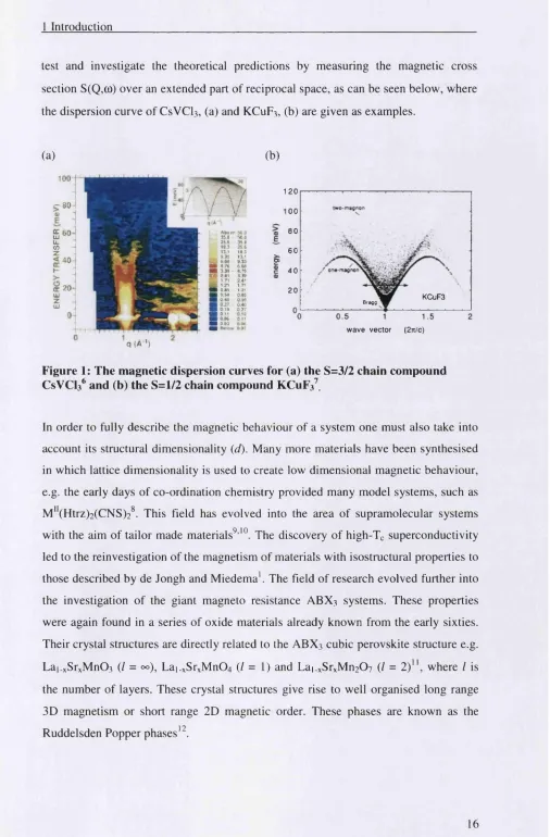
the dispersion curve of CSVCI3, (a) and KCuF^, (b) are given as examples.
(a) (b) looi 5^80
g60-I
<40t-œ 2 0
UJ
z UJ
A b o v r bO.O L 35,« 5 0 0 r a s s 3S.8 ■10.3 25.0 13 1 10 3 9.3S 13.1 _ 6 M 9.15 M 4 M 6.6 0
W m 3.39 4 .M B E 2 4 1 - 3 3 »
1.71 2.41 1 2 1 1 71 ■ I 0.45 1 2 1 m o.sa 0.95 ■ 0.40 0.3» « I 0 2 7 0.40 g 0 1 0 0.27 g 0.11 0 1 8 B 0 06 O i l ■ 0.03 0.06 ■ i 0 03
1 2 0
GO 8 0 6 0 o> 4 0 2 0 KCuF3 B ragg
w ave vector (2ti/c) q ( A ')
Figure 1 : The magnetic dispersion curves for (a) the S=3/2 chain compound CsVCb^ and (b) the S=l/2 chain compound KCuF^^
In order to fully describe the magnetic behaviour of a system one must also take into
account its structural dimensionality (d). Many more materials have been synthesised
in which lattice dimensionality is used to create low dimensional magnetic behaviour,
e.g. the early days of co-ordination chemistry provided many model systems, such as
M"(Htrz)2(CNS)2^. This field has evolved into the area of supramolecular systems
with the aim of tailor made materials^’ The discovery of high-Tc superconductivity led to the reinvestigation of the magnetism of materials with isostructural properties to
those described by de Jongh and M iedem a'. The field o f research evolved further into
the investigation of the giant magneto resistance ABX3 systems. These properties
were again found in a series of oxide materials already known from the early sixties.
Their crystal structures are directly related to the ABX3 cubic perovskite structure e.g.
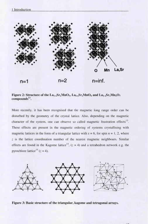
Lai-xSrxMn03 (/ = 00), Lai_xSrxMn04 (/ = 1) and Lai.xSrxMn20v (/ = 2 )" , where / is
the number of layers. These crystal structures give rise to well organised long range
1 Introduction
n=1
n=2
o
Mn
La,Sr
n=inf.
Figure 2: S tru ctu re of the Lai ^Sr^MnO), Lai xSr%Mn0 4 and Lai ^Sr^MniO?
compounds^ \
More recently, it has been recognised that the magnetic long range order can be
disturbed by the geometry of the crystal lattice. Also, depending on the magnetic
character of the system, one can observe so called magnetic frustration effects'^.
These effects are present in the magnetic ordering of systems crystallising with
magnetic lattices in the form of a triangular lattice with z = 6, for spin n = 1,2 , where
z is the lattice coordination number of the nearest magnetic neighbours. Similar
effects are found in the Kagome l a t t i c e(z = 4) and a tetrahedron network e.g. the pyrochlore lattice'** {z = 4).
1 Introduction
The effects of the spin dimensionally, lattice dimensionality and additional frustration
can be directly observed in the critical behaviour around the phase transition
temperature. Phase transitions o f the order - disorder type are characterised by an
order parameter that decreases towards zero with increasing temperature. At a first
order phase transition the order parameter changes discontinuously whereas at a
second order phase transition the change in order parameter is continuous upon
approaching the phase transition from the disordered phase. The magnetic
susceptibility Ôji /ÔH becomes infinite while the magnetic correlation length,
diverges.
In a real system the singularity behaviour of a particular thermodynamic quantity is
limited to a particular region of the phase transition known as the critical region.
Within this critical region the thermodynamic function f(e) often depends on the
reduced temperature e(T - Tc) / Tc as f(e) = Ae^(l+B£^ + ...), where A and B are
constants and x is the critical exponent. The concept and nature o f the different
critical exponents is elaborated upon in Chapter 2. We can say however, that near Tc,
f(e) can be described by a power law ~ Ae* and the value o f x can be obtained from a
‘log - log’ plot of the intensity versus the reduced temperature. The critical exponents
are dependent on the spin dimensionality n, and the system dimensionality d.
Each critical exponent can be expressed as a linear function o f two other exponents
through the laws of scaling the seven scaling relations between the nine critical
exponents are given below:
Y =
Y
a = a '
V = v '
Y = ( 2 -ti)v
a = 2 (l - P ) - y
a = 2 - v d
5 = ( J + 2 -ti) / ( Z > - 2 + ti)
1 Introduction
universal values such as the 2D Ising system where P =0.125 and y = 1.75 or the mean
field predictions of p = Vi and y = 1. These values give us a method of categorising
systems into different universality classes, a topic which is further elaborated on in
Chapter 2. This allows us to predict the behaviour of the system at its phase transition
just armed with knowledge regarding its universality classification. In general, mean
field theory is not valid to describe a phase transition because o f the neglect of very
short range fluctuations. It was shown by Ginzberg, that it was generally inadmissible
to neglect fluctuations with wavelength < The importance o f short wavelength
fluctuations assumes greater importance for reduced lattice dimensionality, since the
energy content o f the fluctuations will be confined to less degrees o f freedom. The
modem renormalisation group theory description of critical phenomena takes the
fluctuations o f smaller wavelengths < ^ into account^
However, it has also been demonstrated by simulation and experimental data that,
depending on the symmetry and spatial geometry within a magnetically ordered
phase, the actual symmetry can be lowered (e.g. by chiral ordering) and new
universality classes may be identified. Thus, it also gives a way to investigate the
changes in critical behaviour by observing the magnetic ordering o f materials with
specific geometry, symmetry and electronic state whilst inducing changes in these
systems by applying electric field (£), magnetic field (H) and external pressure (P).
The study o f differences in the parameters in the Hamiltonian often results in the
study o f a series o f isostructural materials where the changes are induced by the
different crystallographic parameters of the materials in question. Similar changes can
be induced by the application of hydrostatic or uniaxial pressure on a system.
The existence o f spin chirality is still a hotly debated issue. Its existence has been
investigated in this thesis by studying the ABX3 halides using several different routes;
e.g. the application o f external parameters such as electric and magnetic field and
hydrostatic pressure using elastic neutron diffraction as a probe. For the weak Ising
compound CsNiClg we show a transition to chiral ordering by an application of a
magnetic field along the ab plane, (in the spin flop phase the magnetic structure is of
1 Introduction
Using symmetry arguments Plumer et a lP suggested that the application of an
electric field could remove the chirality ordering in the ABX3 ternary halides.
Experimental evidence for this magnetoelectric effect is presented for the compound
CsMnBra. Plumer et al?^ also suggested that a similar chiral ordering should be
observed in the distorted triangular lattice. We have tested this prediction for the
distorted hexagonal perovskite structures of the y - phase o f TlFeClg, in this case we
introduced applied pressure to the system in order to influence the structural
parameters. A test for the existence of chiral order has also been carried out in the P
and y - phases of the distorted hexagonal perovskite KNiClg.
Triangular 120° type magnetic ordering is also induced by an applied electric field: H
// c axis, in the singlet ground state antiferromagnet material CsFeBrs. The critical
behaviour o f the sublattice magnetisation along the phase boundary has been studied
at mK temperatures with applied fields up to 6 Tesla.
Quasi one-dimensional magnetic materials also show interesting and unexpected
magnetic excitations. For example, magnetic soliton motion been observed in ferro as
well as in antiferromagnetic chains e.g. CsNiFs and (CD3)4NMnCl3 (TMMC). For
CsNiCls^^ it was shown that the spin wave description of the magnetic excitation did
not explain the observed energies and intensities. Haldane conjectured that the
magnetic excitations of spins on a 1-D array are different for half integer and integer
spin systems^^’^^. The dispersion of half integer (5 = 1/2, 3 /2 ...) spin chains are
gapless, while the integer spin chains (5 = 1, 2 ...) have a gap at the zone centre. This
gap is related to a singlet —> triplet transition and has been observed in CsNiCl3^^ and
Ni(C2HgN2)N0 2C1 0 4 (NENP)^"^. A schematic of the general phase diagram o f the
anisotropy (Heisenberg —> Ising) versus superexchange (A) for the integer 5 = 1 spin
chains is given below^^. It shows the possible position for a number o f interesting
1 Introduction
RbFel
NENP, KNiCl.
HAF A
Figure 4: Simplified schematic of the phase diagram for the Ising - Heisenberg
chain.
Line 6 in Figure 4 shows the energy of the gap o f the 1-D system versus anisotropy.
The gap energy rises steeply around D = 0. The gap energy in this region corresponds
to the Haldane gap. At high D values this gap goes to zero, as D increases to greater
than 1, the gap opens up again (see Figure 13, Chapter 2.2.1.1). Around the D = 1
point, line 5 in Figure 4 refers to a transition from a singlet ground state to an induced
moment state.
On the antiferromagnet exchange side (right side) o f the phase diagram novel
groundstates were predicted and subsequently found in materials such as NENP and
the ANiCla halides. Experiments have shown that NENP, an S = 1 quasi 1-D system,
shows a gap in the excitation spectrum around the zone centre at Q = 0, which persists
down to low temperatures^"^. In this system the total superexchange ( U ) is smaller
than the crystal field anisotropy (D). The observed gap energies are well explained by
Haldane’s predictions. However, for other systems shown in Figure 4, there are
further complications, as in the case of CsNiClg where magnetic order takes place. In
this case the superexchange is much larger than the anisotropy of the system. It was
shown that the spinwave description of the magnetic excitations does not explain the
observed energies and intensities o f these excitations. CsNiClg has two modes present
in the dispersion curve of the magnetic excitations; a linear mode which decreases to
1 Introduction
have a quantum mechanical origin. Very few materials are available to investigate the
effect o f different amounts of anisotropy on the S = 1 linear chain compounds.
However a tuning of the gap mode is made possible by applying an external pressure
on the system. In Appendix A, the dispersion of the magnetic excitations o f the weak
Ising like systems CsNiClg and RbNiClg under an applied hydrostatic pressure of
5kbar are presented, these have not been treated and are given ‘as is’. The dispersion
of the magnetic excitations in the XY like quasi one-dimensional linear chain
compound KNiCls has also been investigated in its p and y - phases. These results are
presented in Chapter 4.5.
The position o f the quasi one-dimensional AFeXg compounds is also indicated on the
phase diagram in Figure 4. In these materials one finds that the magnetism at low
temperatures is governed by the singlet ground state and the low-lying doublet state.
This can be described by an effective S = I Hamiltonian. The full spin moment is
actually 5 = 2. The anisotropy in the AFeXg systems is much higher than that in the
ANiX] ones^^. Singlet ground state (SGS) behaviour is observed in the CsFeX] (X =
Cl, Br), whereas the RbFeX] compounds have an induced moment behaviour and the
systems order magnetically at low temperature. This is due to the fact that in the
CsFeX] compounds, D > S / and for the RbFeXg compounds, D <1L J. The small
differences apparent in the values of the anisotropy and intra- and interohdim
superexchange is caused by the small variation in the structural parameters o f the
systems.
Applied hydrostatic pressure on the CsFeX] compounds has been explored as a means
of inducing magnetic order in the system. A magneto-structural study of the systems
is presented in Chapter 5. The dispersion of the magnetic excitations o f CsFeClg and
CsFeBrs are measured as a function o f applied hydrostatic pressure (up to 5kbar) at
low temperature (< 2K). The corresponding crystal structures are also determined by
means o f time-of-flight neutron diffraction measurements. Magnetic order can also be
induced in these compounds by application of a magnetic field along the chain
direction. In this case the low-lying doublet (m = ±1), is Zeeman split and for a
sufficiently large field the lower doublet state (m = -1), will approach and eventually
1 Introduction
structure. The dispersion o f the magnetic excitations are studied for the Singlet
Ground State (SGS) antiferromagnet CsFeBrs for very low temperatures (60mK) in
the presence o f a magnetic field (5T) and presented in Chapter 5.3. Up to the phase
transition an accurate description o f the dispersion is given by the theory o f Lindgârd
while in the ordered state the Dynamical Correlated Effective Field Approach
(DCEFA) o f Suzuki is preferred“ ’^’’^*.
The thesis is arranged in the following order; Chapter 2 is presented as the theory
chapter. Within this chapter structural and magnetic information is given on the
diverse ABX3 family o f compounds and reasons for studying them are elaborated
upon. The chapter also contains the necessary neutron scattering theory for the reader
to understand experimental evidence given in later chapters. As this thesis deals
specifically with experiments on the ABX3 compounds, and as such, is an
experimental thesis as opposed to a theoretical one. Chapter 3 gives information on
the crystal growth and experimental methods employed in this thesis as well as
individual specification of spectrometers and diffractometers used to collect data on
the systems. The actual experimental results are presented and discussed in Chapters 4
and 5. Chapter 4 deals with chirality order in the ABX3 compounds and Chapter 5
looks at the SGS compounds CsFeCl3 and CsFeBr3. A summary of results and a
statement of further work is outlined in Chapter 6. Finally, Appendix A deals with
recent experimental findings from the magnetic excitations of the easy axis
compounds CsNiCl3 and RbNiCl3 under applied hydrostatic pressure, as well as those
2 Theory___________________________________________________________________
2 Theory
This Chapter introduces the ABX3 halides and classifies them according to the
strength o f their chainar anisotropy. Each classification is elaborated upon and
information is given on their structural and magnetic properties. The theory behind
universality, critical phase transitions and the production and diffraction o f neutrons is
also given herein.
2.1
Second Order Phase Transitions.
In this thesis a series o f magnetic materials are studied which show magnetic ordering
upon the application of magnetic field, electric field or applied pressure or by the
lowering o f the temperature o f the system. Systems which undergo a second order
phase transition, i.e. a transition where the second derivative o f the Gibbs free energy
changes discontinuously are said to have undergone a critical phase or continuous
phase transition. To explain the concept of critical behaviour at phase transitions it is
probably best to consider the phase transition of a simple ferromagnetic system. The
typical magnetisation, M, of a simple ferromagnet, under different temperature
conditions follows the form o f that given below. The behaviour can be described by
simple m olecular field theory, which can be found in many general physics textbooks.
The relative magnetisation o f the system ( a = M/Mo where Mo is the magnetisation at
T = OK) is modelled by the equation:
o = B j gH^( H + X a )
kgT
(2)
where the Brillouin function Bj is given by:
_ , \ 27 + 1 j 2 J + l \ 1 r X "I
coth X coth —
" ^ ^ 2 7 i 27 j 27 ( 2 7 ^
2 Theory___________________________________________________________________
Close to the phase transition a is small and Bj can be expanded in a power series of
g/igAcr/ksT. In the first approximation:
=
(4)
we see from this expansion that the transition to the paramagnetic phase (cr = 0) takes
place at:
Just below Tc the magnetisation behaves according to:
a = A ( ( T c - T ) / T c f (6)
where mean field theory predicts that P = 0.5. Similarly one can calculate the
magnetic susceptibility, % = M / H , above giving us:
X = A ' ( T - T J ^ (7)
where mean field theory predicts that y = 1.0. A full breakdown of the critical
2 Theory_______________________________________________________________
Table 1: Definition and range of values for critical exponents encountered in
Table 2 and Table 3.
Thermodynamic Variable
Sym bol Power Comments Typical values
o f exponents Specific Heat at Ch ( T - T J ^ T > T „ H = 0 -0.3 - 0.3
Constant field ( T c - T ) - " ' T < T „ H = 0 -0.3 - 0.3 M agnetisation M ( T , - T f T < T c , H = 0 0.1 - 0 . 4
fjl/S T = T c 3 . 0 - 6 . 0
Susceptibility X ( T - T , f T > T c , H = 0 1 . 3 - 1 . 4 T < Tc, H = 0
Correlation ( T - T J ' T > T c . H = 0 0.6 - 0.7
Length ( T , - T r ' T < T c , H = 0 0.6 - 0.7
The values o f the critical exponents for magnetisation {p and Ô) and for correlation
length (v) can be obtained by neutron scattering and the critical exponents for
susceptibility (y) can be obtained from AC measurements. As has been mentioned in
the Introduction, the critical exponents are linked by scaling laws. The values of the
critical exponents allow us to establish the universality class of the system.
According to the universality hypothesis, second order phase transitions may be
classified as belonging to a small number of universality classes. The class to which
the system belongs depends on a small number of basic properties o f the system:
• The spatial dimension of the system, (c? = 1,2 or 3 dimensional)
• The spatial dimension or symmetry of the order parameter, (Ising, XY and
Heisenberg for w = 1 ,2 and 3 dimensions respectively)
• W hether the order parameter is short or long range.
This is rather astonishing as it represents quite a large generalisation. It implies that
the nature of the microscopic interaction is irrelevant (aside from the last point). It
also implies that for continuous transitions such as magnetic transitions, the critical
2 Theory___________________________________________________________________
Therefore armed with the above knowledge, one can classify the universality o f a
system and thus define the universal qualities such as critical components, amplitude
ratios and equations of state. If one concentrates on a standard bulk magnet, one sees
that the universality o f the system is basically determined by the symmetry of the
order parameter. The critical properties associated with these n-component, 0(n),
universality classes have been extensively studied and are well understood. The
values for the critical exponents for the different standard models are given below.
Table 2: Critical exponent values for the standard universality classes
Standard M odel
Universality Class
a P Y v
A+/A-Ising Z2 0.1098(29) 0.325(1) 1.2402(9) 0.6300(8) 0.55
X Y SI -0.0080(32) 0.346(1) 1.3160(10) 0.6693(10) 0.99
Heisenberg S2 -0.1160(36) 0.3647(12) 1.3866(12) 0 .7054(11) 1.36
However, there are systems which fail to be represented by the standard 0 (« )
universality classes, systems such as random magnets with quenched disorder (e.g.
spin glasses). Other systems include those standard magnets with frustrated
magnetism. The nature of frustrated magnets leads to quite new and exciting phase
transitions to those of conventional unfrustrated magnets, as will be demonstrated in
what follows.
In order to understand the concepts of the standard magnets with frustrated
magnetism, let us consider a triangular lattice with antiferromagnetically coupled
spins at each vertex. It is immediately apparent that the spins cannot conform to a
collinear antiferromagnetic alignment, the stable spin configuration depends on the
type of spin symmetry or number of spin components. In the case of the spins being
confined to one dimension (called the Ising case) the ground state is not uniquely
2 Theory
Ü ?
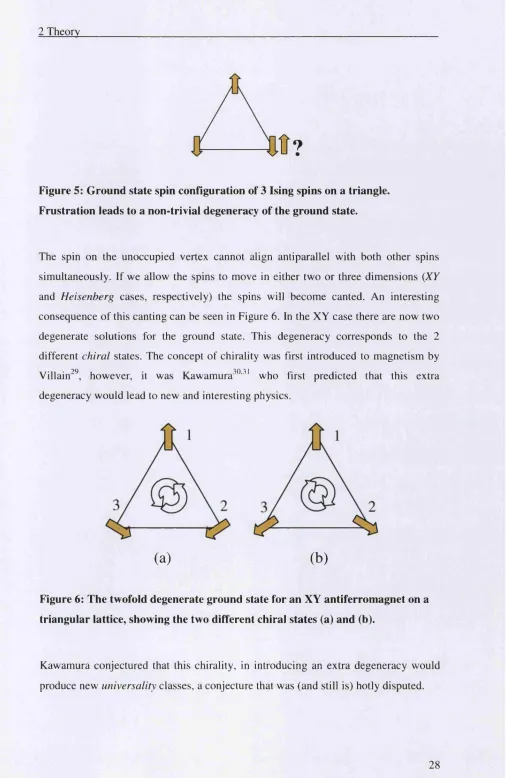
F igure 5: G ro u n d state spin co nfiguration of 3 Ising spins on a triangle.
F ru stra tio n leads to a non-trivia! degeneracy of the g ro u n d state.
The spin on the unoccupied vertex cannot align antiparallel with both other spins
simultaneously. If we allow the spins to move in either two or three dimensions {XY
and Heisenberg cases, respectively) the spins will become canted. An interesting
consequence of this canting can be seen in Figure 6. In the XY case there are now two
degenerate solutions for the ground state. This degeneracy corresponds to the 2
different chiral states. The concept of chirality was first introduced to magnetism by
Villain^^ however, it was Kawamura^"'^' who first predicted that this extra
degeneracy would lead to new and interesting physics.
(a)
(b)
F igure 6: T he tw ofold d egenerate g ro u n d state fo r an XY a n tiferro m ag n e t on a
tria n g u la r lattice, show ing the two different ch iral states (a) a n d (h).
Kawamura conjectured that this chirality, in introducing an extra degeneracy would
2 Theory___________________________________________________________________
It can be seen from Figure 6, that a given chiral state cannot be transformed to the
other chiral state via a global spin rotation in the X V spin space. It is necessary to use
global spin reflection to achieve this. One may assign a different chirality o f plus (+)
or minus (-) to (a) and (b) in the above figure. Thus the extra degeneracy provide by
the chiral states manifests itself as a hidden Ising like degeneracy. In order to
characterise these two chiral states it is convenient to introduce a scalar quantity,
chirality^^,
3V3
É
{ij)[^,X 5,1
= 3V3 {ij) - S I S ' )= I f )(8)
where the sununation runs over the 3 spins depicted above. Kp = ± l for the two spin
configurations.
Looking at the Heisenberg case, we see that there is no longer a discrete chiral
degeneracy as the different spin configurations can be transformed into one another
by continuous spin rotation via the third dimension. However, a chirality vector can
be defined as.
(9)
A similar chiral degeneracy may be observed in systems such as helimagnets and 2D
and 3D stacked triangular lattice antiferromagnets, the spin structures o f which are
shown below.
2 Theory___________________________________________________________________
Kawamura first analysed the critical properties of systems known as stacked
triangular lattice antiferromagnets (TLA’s), this being the antiferromagnetic stacking
o f the triangular lattice seen in Figure 7. Kawamura used the theoretical techniques of
symmetry analysis and Monte Carlo simulation to show that due to this extra chiral
degeneracy, TLA systems may belong to a new universality class. The critical
exponent values obtained by Kawamura for his new universality class are listed below
and can be compared with the standard universality class critical exponents in Table
2.
Table 3: Critical exponent values for the chiral universality classes.
Chiral Universality a P y V aVa
-Model Class
X Y Z 2 x S l 0.34(6) 0.253(10) 1.13(5) 0.54(2) 0.36(2)
Heisenberg P3 0.24(8) 0.30(2) 1.17(7) 0.59(2) 0.54(2)
In order to investigate the Kawamura hypothesis it is necessary to find model systems
with antiferromagnetic triangular lattice structures. Two such groups that satisfy this
criteria are the BX2 and ABX3 halide families, where A is a lA group cation, B is a
divalent first-row transition metal cation and X is a halide anion. A wide variety of
magnetic properties may be obtained by changing the B ion (due to the electronic
changes induced) and the A and X ions (due to spatial changes). The different
properties obtainable are due to the change in geometry and nature of the
superexchange bridges, and the different electronic states induced by the crystal field
levels for different types o f B ion.
These systems generally crystallise in the hexagonal perovskite structure with space
group Pbs/mmc. Chains of face-sharing B X ^ octahedra aligned along the c-axis are
separated by the ions. This results in the interchsm separation being much larger
than the /nrrachain separation, leading to a quasi one-dimensional magnetic behaviour
2 Theory
Figure 8: Schematic of the hexagonal perovskite structure, with the ions
separating the infinite linear chains of BXl~ face-sharing octahedra, space
group PéVmmc.
Figure 9: [0001] projection of hexagonal perovskite structure. The hexagonal
stacking of the tw inned-cuboctahedral AXn coordination polyhedra, which
2 Theory
2.2
Heisenberg Triangular Antiferromagnets
This Chapter gives a brief overview of the family o f Heisenberg triangular
antiferromagnets. It introduces the systems reported on later in the thesis and acts as a
reference point to the reader. It is by no means comprehensive and the interested
reader is referred to the recent review by Collins and Petrenko^^
Figure 10: A schematic of the stacked triangular antiferromagnet lattice.
The stacked triangular antiferromagnet takes the form as that shown in Figure 10, it
can be described with the following Hamiltonian:
d»f’ = j ' ^ S , S j + r ' ^ S , S j
(
10
)
1<J 1<J
Where J is the exchange integral along the chains, J ' is the exchange integral between
the chains and D is the single ion anisotropy. The first term represents the
superexchange parameter along the chain, the second term represents the