Weighted Round Robin Configuration for
Worst-Case Delay Optimization in Network-on-Chip
Fahimeh Jafari
∗, Axel Jantsch
†, and Zhonghai Lu
‡ ∗Liverpool Hope University, UK†TU Wien, Vienna, Austria
‡KTH Royal Institute of Technology, Sweden
Abstract—We propose an approach for computing the end-to-end delay bound of individual variable bit-rate flows in a FIFO multiplexer with aggregate scheduling under Weighted Round Robin (WRR) policy. To this end, we use network calculus to derive per-flow end-to-end equivalent service curves employed for computing Least Upper Delay Bounds (LUDBs) of individual flows. Since real time applications are going to meet guaranteed services with lower delay bounds, we optimize weights in WRR policy to minimize LUDBs while satisfying performance constraints. We formulate two constrained de-lay optimization problems, namely, Minimize-Delay and Multi-objectiveoptimization.Multi-objectiveoptimization has both total delay bounds and their variance as minimization objectives. The proposed optimizations are solved using a genetic algorithm. A Video Object Plane Decoder (VOPD) case study exhibits 15.4%
reduction of total worst-case delays and 40.3% reduction on the variance of delays when compared with round robin policy. The optimization algorithm has low run-time complexity, enabling quick exploration of large design spaces. We conclude that an appropriate weight allocation can be a valuable instrument for delay optimization in on-chip network designs.
Index Terms—Network-on-chip, performance evaluation, net-work calculus, worst-case delay optimization, weight configura-tion.
I. INTRODUCTION
Many multi-core Systems on Chip (SoC) require different levels of service for different applications. Real-time applica-tions have stringent performance requirements; the correctness relies not only on the communication result but also the end-to-end delay bound. A data packet received too late could be useless. In other words, the Least Upper Delay Bound (LUDB) for each packet must not exceed its deadline. In such systems, it is desirable to minimize the end-to-end delay bound of the traffic streams satisfying their QoS requirements. Therefore, the first important consideration is to derive the LUDB for a given communication flow. To this end, based on the Network Calculus theory [1], we have presented and proved required theorems in [2] [3]. We then presented a methodology [4] to consider resource sharing scenarios and also derive end-to-end Equivalent Service Curve (ESC) and LUDB by applying the proposed theorems. We assume that all traffic can be well characterized as flows and scheduled as aggregates which means multiple flows are scheduled as an aggregate flow. For a given flow, we study the maximum interference of all other flows based on the Network Calculus. Our proposed models [4] have been defined and validated under Round Robin (RR) policy. RR policy uses the same service level for each connection while multiple service levels allow to better adapt to the application requirements by providing different
bandwidth and latency guarantees. A Weighted Round Robin (WRR) scheduling policy assigns weights to concurrent com-munications to define multiple service levels. Higher service levels have greater weights and do not preempt lower ones. It is important for designers to find appropriate weights in WRR policy such that the corresponding service levels can support QoS requirements for each communication connection. It is desirable to also optimize delay and throughput in the network.
In this paper, we extend our earlier proposed methodology for RR [4] to WRR policy. We then address an optimization problem of minimizing the total delay bounds subject to the performance constraints of the applications running on the SoC. To avoid unfair services, we consider another objective for minimizing the variance of delay bounds in different flows. Minimizing the variance of the delay bounds avoids an intolerable delay of some flows, caused by processing and transmission of other flows. As both mentioned objective func-tions are important for the real-time applicafunc-tions, we formulate them as a multi-objective problem under QoS constraints. Finally, we show the benefits of the proposed method and quantify performance improvement.
Random variables appear in the formulation of the optimiza-tion problem which causes random objective funcoptimiza-tions. Such optimization problems are usually solved by metaheuristic methods which do not guarantee an optimal solution. However, they usually find high-quality solutions in reasonable time [5]. There is a wide variety of metaheuristics like simulated annealing, tabu search, iterated local search, evolutionary computation, and genetic algorithms. We compare the perfor-mance of several metaheuristics (pure random search,markov monotonous approach,adaptive search, andgenetic algorithm) and conclude that a genetic algorithm based method is most suitable.
II. RELATEDWORK
A. Performance Evaluation of Real-time Services
There are different mathematical formalisms for perfor-mance evaluation in on-chip networks. We have surveyed four popular techniques along with their applications and also reviewed their strengths and weaknesses [6]. Most of the current works use queuing theory-based approaches. For example, Ben-Itzhak et al. [7] propose an analytical model for deriving the average end-to-end latency and link utilization of wormhole NoCs with heterogeneous link capacities and heterogeneous number of virtual channels per unidirectional link. Queuing approaches often use probability distributions like Poisson to model traffic in the network while Poisson distribution is not appropriate for characterizing all traffic patterns in NoC applications. Qian et al. [8]–[10] suggest a methodology for addressing the limitation of assuming traffic arrivals as Poisson processes. They present analysis for a general arrival process based on G/G/1 queue model [9]. In SVR-NoC [8] [10], the proposed analytical model is embedded into the learning process to form the feature vectors and in turn consider a more generalized traffic model. Although queuing approaches have been widely used for performance analysis, they cannot properly model some significant features, such as nonstationary, self-similarity, higher order statistics, for NoC-based multicore platform designs. To overcome this limitation, Bogdan et al. [11] suggest an approach which analyzes the traffic dynamics and captures the non-stationary effects of the NoC workload. They propose QuaLe model [12] based on statistical physics to analyze the information flow and buffer usage in NoCs, and also investigate the impact of packet injec-tion rate and data packet sizes on the multi-fractal spectrum of traffic. In following up to this work, Bogdan et al. [13] propose mathematical frameworks for exascale computing in data-centers-on-a-chip architectures that exploit the NoC paradigm for interconnecting large number of heterogeneous processing elements. The frameworks can account and exploit the non-stationary and multi-fractal characteristics of computation and communication workloads. To address the problem of distant and large volume data exchange, Xue and Bogdan [14] present a user-cooperation network coding strategy for NoCs.
Network calculus is another mathematical approach special-ized for deriving worst-case performance analysis. Network calculus is able to model all traffic patterns with bounds defined by arrival curves. It provides the facility of capturing dynamic features of the network based on the traffic flows’ shapes. Network calculus has been applied in a number of papers for performance analysis of real-time services in networks with aggregate scheduling. For example, Charny and Boudec [15] derive a closed-form delay bound in a generic network assuming a fluid model. An extended model is proposed [16] to look into packetization effects. The main limitation of these models is that they work well only for small utilization factors in a generic network configuration. Lenzini et al. [17] describe a methodology for obtaining per-flow worst-case delay bound in tandem networks of rate-latency nodes traversed by leaky-bucket shaped flows. This method yields better bounds than those previously proposed. Qian et al. [19] present analytical
models for traffic flows under strict priority queueing and weighted round robin scheduling in on-chip networks. They then derive per-flow end-to-end delay bounds using these models.
All previous works based on network calculus investigate computing delay bounds only for average behavior of flows and they do not consider peak behavior, which results in less accurate bounds. Since a considerable number of real time ap-plications are transmitted by Variable Bit-Rate (VBR) traffics, we have proposed a methodology [4] to consider performance analysis for VBR traffic characterized by(L, p, σ, ρ)in on-chip networks employing aggregate resource management. This method achieves more accurate delay bounds. In this paper, we extend this method to WRR and then regulate weights in each router to minimize delay bounds while satisfying performance constraints.
B. Performance Improvement
There exist some previous related works focused on flow-control, adaptive routing, and also domain isolation based on non-interfering router microarchitecture. Concer et al. [20] pro-pose an end-to-end flow control protocol, called Connection-Then-Credit (CTC), to handle message-dependent deadlocks in on-chip networks. Although this protocol adds a latency overhead to the transfer of the message, under some conditions, the performance of the system can be improved. As CTC is an extension to the normal credit-based flow control protocol, Sallam et al. [21] implement both protocols and investigate implementation trade-offs along with performance analysis. Joshi and Mutyam [22] consider a prevention flow control mechanism which satisfies cost/performance constraints in torus networks while preventing deadlocks by combining pri-ority arbitration with prevention slot cycling. However, the mechanism can lead to deadlocks with variable-sized packets. There are a wide range of adaptive algorithms varying from partially to fully adaptive and have the potential for improving system performance [23]–[26]. For instance, Lin and Tang [23] develop a bufferless routing algorithm and have shown improvements of up to 10% for average latency when com-pared to older designs. Najib et al. [24] present a look-ahead partial adaptive routing for their prior proposed low-latency NOC router [27]. They show that their algorithm improves the performance of a baseline design of the router under imbalanced traffic. Sheng et al. [25] [26] propose a flow control technique, called Whole Packet Forwarding, which is a VC re-allocation scheme for fully adaptive routing in wormhole on-chip networks. They show that fully adaptive routing can offer higher performance than several partial adaptive routing algorithms.
pipeline and at the network level. They also design appropriate scheduling of flows to reduce area/delay cost in the network.
All above mentioned works consider reducing average la-tency in different system models while, in this paper, we calculate worst-case delay bounds under WRR scheduling policy and deterministic routing and minimize worst case delay and variance.
III. NETWORKCALCULUSBACKGROUND
Network calculus is a mathematical approach to compute worst case bounds for guaranteed services in communication networks [1]. It uses min-plus algebra to convert non-linear queueing systems into linear systems. The algebra structure of min-plus is (< ∪ {+∞},∧,+) in which ∧ represents the minimum operation, f ∧g = min(f, g). The min-plus convolution, denoted by ⊗, is defined as (f ⊗ g)(t) = inf0≤s≤t{f(t−s) +g(s)}; where two functionsf andg are
wide-sense increasing functions.
An arrival curve defines an upper bound on the cumulative arrival process to characterize a traffic flow and a service curve defines a lower bound on the cumulative service process. In this paper, we use Traffic SPECification (TSPEC) [35] for characterizing traffic to look into both the average and peak behaviors of a flow. With TSPEC, the arrival curve of flow fj is defined as αj(t) = min(Lj+pjt, σj+ρjt) in which Lj is the maximum transfer size, pj the peak rate(pj≥ρj), σj the burstiness (σj ≥Lj), andρj the average (sustainable)
rate. We denote it asfj ∝(Lj, pj, σj, ρj). A well-formulated
service model to reflect the service capability of a node is the rate-latency function defined as βR,T = R(t − T)+,
where R is the minimum service rate and T the maximum processing latency of the node. We use x+ to denote the function x+ =x if x > 0;x+ = 0, otherwise. ∨ represents the maximum operation, f ∨g = max(f, g). Burst delay function δT(t) = +∞, if t > T; δT(t) = 0, otherwise.Affine
function γb,r(t) = b+rt, if t > 0; γb,r(t) = 0, otherwise.
Therefore,δT ⊗γb,r(t) =b+r(t−T).represents the
min-plus deconvolution as(fg)(t) =sups≥0{f(t+s)−g(s)}.
IV. SYSTEMMODEL
We consider a Network-on-Chip (NoC) architecture in which every node contains a core equipped with a Network Interface (NI) and a router with input and output channels. Assumptions are given as follows:
• The NoC architecture can have arbitrary topologies.
• A flow consists of packets and each packet is broken
into flits. We consider thearbitration granularity of one word with a fixed word length ofLwfor all flows.Lwis
assumed to be1 flit.
• Packets have fixed length and traverse the network in a best-effort fashion with virtual-cut-through switching technique using deadlock-free deterministic routing.
• Routers have multiple flit input buffers but no output buffers.
• The router can have multiple Virtual Channels (VCs) per in-port. VC allocation is deterministic and each VC receives an aggregate service.
4 r 1
r r2 r3
8 r 6
r r7
5 r
9 r
2 f
1 f
4 f 3 f
13
r r16
10
r r11
9
r r12
15 r 14
r
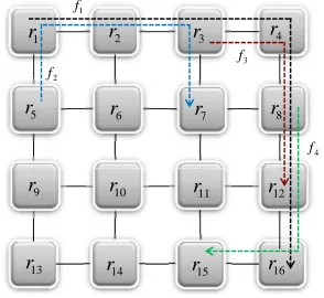
Fig. 1. An example of a NoC with16nodes and4flows.
• Buffers are bounded by Eq. (7) and the network is
lossless.
• All traffic is modeled as TSPEC flows f = T SP EC(L, p, σ, ρ)at the entry into the network.
• To characterize flows based on TSPEC, we assume un-buffered leaky bucket controllers (regulators) which do not buffer the packets, but stall the traffic producers or IPs [18].
• We assume weighted round robin arbitration and model it by a rate-latency service curve asβ =δT ⊗γ0,R, it is
assumed that ρ≤R andp≥R, whereρis the average rate,pthe peak rate, andR the minimum service rate.
• Flows are classified into a pre-specified number of ag-gregates and traffic of each aggregate is buffered and transmitted in FIFO order, denoted as FIFO multiplexing.
• Different aggregates are buffered separately and each
aggregate is guaranteed a rate-latency service curve.
• The hardware limits the peak rate to1 flit/cycle.
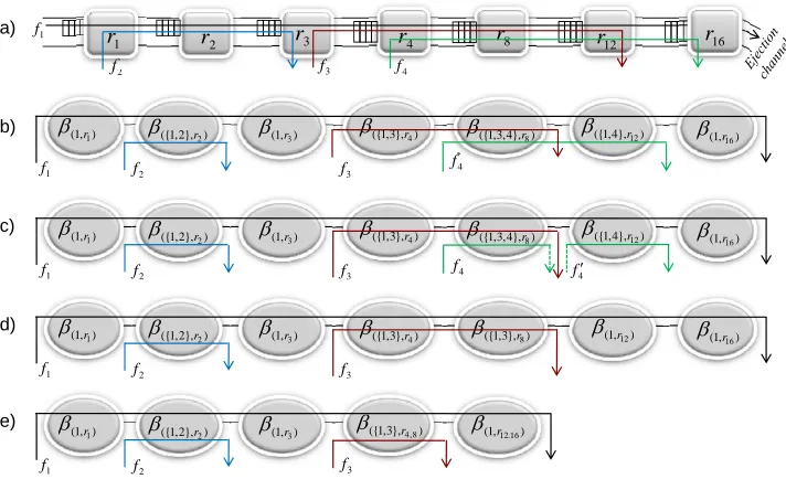
Figure 1 depicts an example with 16 nodes and 4 flows. Multiple flows which share the same buffer and channel in the same router, for examplef1andf2 in router2, are scheduled as an aggregate flow denoted as f{1,2}. The tagged flowis a
flow for which the delay bound is derived and the other flows which compete with the tagged flow for the same resource are calledcontention flows. In the example, iff1is the tagged flow,f2,f3, andf4would be contention flows. Table I presents notations in this work.
Sub-indices ”(fi, rj)” indicate that they are related to flowfi
in router rj. For instance, α(f1,r2) indicates the arrival curve
of f1 in router r2. Using fsi instead of fi in the sub-index
means that the notation is related to thefsi which can be one
flow or an aggregate flow. For example, β({1,2},r2) refers to
aggregate flowf{1,2} in routerr2.
V. LUDB DERIVATION FORWRR POLICY
TABLE I THE LIST OF NOTATIONS
fi Flowi
FRP V (j,i,k)
The set of flows passing through VCkin physical channeliof routerj
F(j,l,s,k) The set of flows passing from VCchannellto output channelkin routersof inputj
Input PC# The number assigned to an input physical channel
Output PC# The number assigned to an output physical channel
VC# The number assigned to an input virtual channel InP C The set of input physical channels in each router OutP C The set of output physical channels in each router
InV C The set of input virtual channels in each inputphysical channel
Li The maximum transfer size offi(flits)
pi The peak rate offi(flits/cycle)
σi The burstiness offi(flits)
ρi The average rate offi(flits/cycle)
Src(i) The source node offi
rj Routerj
βj The service curve ofrj
R The minimum service rate in a rate-latency service curve
Tl The maximum processing latency of the arbiter in
the router(cycles)
THoL The maximum waiting time in the FIFO queue of
the router(cycles)
TT otal The total processing delay which comes from contention
flows the router and equals to the sum ofTlandTHoL
Drouter Time spent for packet routing decision(cycles)
Lw The word length in the flow(flits)
C The channel capacity(flits/cycle)
CFt The set of contention flows of tagged flowft
si
The set of joint flows in an aggregate flow (when the number of elements ofsiis equal to1,
there is only a single flow) fsi An aggregate flow ofsi
|si| The cardinality of setof the ”number of elements of the set”si, which is a measure
F(Bs
i,rj)
The set of flows which share the same buffer in routerrjwith flowfsi
w(j,l,s,k)
The weight assigned to noderj, input Physical
Channel (PC)l, input VCs, and output PCk LW R The length of a round in WRR policy
To this end, we propose the two following steps to derive the end-to-end service curve for a tagged flow:
• Step 1: Intra-router ESC: This step derives intra-router
ESCs for each router through which the tagged flow is passing. Different resource sharing scenarios in each router are distinguished and intra-router analysis models are built.
• Step 2: Inter-router ESC: In this step, according to the intra-router analysis models, we present a set-theoretic approach which recognizes and investigates different con-tention scenarios that a flow may experience along its routing path and in turn derive an end-to-end ESC for the tagged flow.
For extending our proposed analytical method to weighted round robin policy, we expand the first step while the second step is unchanged. Similarly, to support some other arbitration policies, only the first step must be modified.
A. Intra-router ESC
In this step, we consider three types of resource sharing, including channel&buffer sharing, channel sharing, and buffer sharing.
1 f
2 f
D
E
M
U
X
PC
PC 1,2
f
D
E
M
U
X
Fig. 2. An example of channel&buffer sharing
D
E
M
U
X
2 f
1 f
DEMUX
Input PC#1
Input PC#2
Output PC #1
VC#0
VC#0 VC#1
PC
D
E
M
U
X
VC#1
Node#3
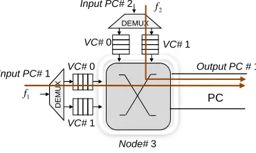
Fig. 3. An example of channel sharing
1) Channel&Buffer Sharing: As shown in Figure 2, mul-tiple flows share both the same buffer and channel in the router, and are scheduled as a flow called aggregate flow. An aggregate flow including the tagged flow is named as tagged aggregate flow. In this case, intra-ESC is derived for the tagged aggregate flow instead of the tagged flow. In Section V-B, due to contention scenarios, we will remove contention flows from the ESC of a tagged aggregate flow in order to extract the ESC of the tagged flow.
2) Channel Sharing: Figure 3 depicts an example of a channel shared between two flowsf1andf2. The WRR arbiter associates a weightw(j,l,s,k)in cycles on each aggregate/single flow fsi passing from input VC s of input Physical Channel
(PC) l in router rj to output PC k. The value of the weight
assigned to a channel depends on flows passing through that channel. Then, the router will try to give the flow a period of w(j,l,s,k)cycles before moving to the next node. In each round, for a non-empty VC buffer encountered, the router serves up to corresponding configured weight in cycles. The maximum length of a round consequently equals toP
l,sw(j,l,s,k)cycles, denoted asLW R. The least service offered to one flow in a VC
is completely dependent on the weight of that VC and the sum of all other weights. With the WRR scheduling, the worst case appears for a flow when it just misses its slot in the current round. Consequently it will have to wait for its slot assigned at the next round. In the worst case, each flowfsi passing from
input VCsof input PCl in routerrjto output PCkwill have
to wait up toP
p,qw(j,p,q,k)−w(j,l,s,k)
× Lw
C +Drouter
cycles before to be served, and get at least a w(j,l,s,k)
P
p,qw(j,p,q,k)×C
PC 1 f 2 f P C D E M U X P C 1 f 2 f 0 ) , ( ) , ( 1 1 l r f r f T C R 0 ) , ( ) , ( 2 2 l r f r f T C R P2 P2 P2 P2 ... P2 P2 P1
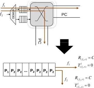
Fig. 4. An example of buffer sharing
Lw the word length, andDrouterthe delay for packet routing
decision in a router. A flow may get more service rate if other flows use less, but we now know a worst-case lower bound on the bandwidth. Based on network calculus theory, we can use the abstraction of service curve to model a weighted round robin arbiter in router rj for flowfsi as a rate-latency
server β(si,rj)=R(si,rj)(t−T
l
(si,rj))
+, whereR
(si,rj) is the
minimum service rate andTl
(si,rj)is the maximum processing
latency of the arbiter in router rj for flow fsi. R(si,rj) and
Tl
(si,rj)are defined as follows:
R(si,rj)=
w(j,l,s,k) P
p,qw(j,p,q,k)
×C (1)
T(ls
i,rj)=
X
p,q
w(j,p,q,k)−w(j,l,s,k) !
×
L
w
C +Drouter
(2) In the example of Figure 3:
R(f1,r3)=
w(3,1,0,1)
w(3,1,0,1)+w(3,2,1,1) ×C
T(lf
1,r3)=w(3,2,1,1)× Lw
C +Drouter
As aforementioned, the sum of weights of flows sharing a channel is equal to the round time. Thus, as the value of round time (the sum of weights) is increased or decreased, individual flows proportionally get more or less time slots respectively, which means the weights proportionally increased or decreased. Therefore, the model is able to adjust the weights based on the round time.
3) Buffer Sharing: Figure 4 depicts a buffer shared between two flowsf1andf2. In this type of sharing, we introduce two kinds of delay for a tagged flow including:
• Head-of-Line delay (HoL) is the maximum waiting time of the packet in the FIFO queue, which is denoted by THoL.
• Processing delay is the maximum processing latency of the router’s arbiter for the flow, which is denoted by Tl.
Therefore, total delay for tagged flow fi in router rj is
calculated as T(T otalf
i,rj)=T
HoL
(fi,rj)+T
l
(fi,rj).
Tl
(fi,rj)andR(fi,rj)can be calculated according to Equation
(2) and (1), respectively. To show how THoL
(fi,rj) is calculated,
we consider the example in Figure 4 and assume thatf1is the tagged flow. As depicted in the figure, THoL
(f1,r) is equal to the
maximum delay for passing packets of flow f2 in the buffer. According to [1], the maximum delay for flowfj is bounded
by Equation (3).
¯
D(fj,r)=T
l
(fj,r)+
Lj+θj(pj−R(fj,r))
+
R(fj, r)
(3)
whereθ= (σ−L)/(p−ρ). Therefore,T(HoLf
1,r) is given as follows:
T(HoLf
1,r)=T l
(f2,r)−θ2+
L2+θ2p2
R(f2,r)
(4)
In the case of more than one flow sharing the same buffer with the tagged flow, HoL delay for tagged flowfsi in router
rj is calculated as below:
T(HoLsi,rj)= X
∀fc∈F(Bsi,rj)
THoL(fc)
(si,rj) (5)
whereFB
(si,rj)is the set of flows which share the same buffer
in routerrj with tagged flowfsi. AlsoT
HoL(fc)
(si,rj) is given by
THoL(fc)
(si,rj) =T
l
(fc,r)−θc+
Lc+θcpc R(fc,r)
(6)
Therefore router rj can give flow fsi service bounded by
curve β(si,rj)=δT(T otalsi,rj) ⊗γ0,R(si,rj), where T T otal
(si,rj) is equal
toT(HoLs
i,rj)+T
l
(si,rj)andR(si,rj)is calculated by Equation (1).
We analyze the buffer space threshold for each VC based on traffic specifications of flows passing through that VC, and also interference between them. The buffer space threshold for virtual channelkin physical channeli of routerj is given as below:
B(j,i,k)= X
∀fc∈F(RP Vj,i,k)
σc+ρcT(pf
c,rj)+
θ−T(pf
c,rj)
+
×h pc−R(fc,rj)
+
−pc+ρc
i
(7) whereFRP V
(j,i,k) is the set of flows passing through VCk in physical channel iof router j.
B. Inter-router ESC
In this step, we aim to extract ESC of the tagged flow by removing the contention flows from the ESC of the tagged aggregate flows. We have described this stage in elaborate detail through our previous paper [4]. For the sake of complete-ness, it is explained in the appendix. Algorithm 1 presents the main steps of deriving the end-to-end ESC for a given tagged flow. The only difference between this algorithm and the one presented for RR [4] results from the different methods pro-posed for calculating intra-router ESCs (Line9). The algorithm with all stages, including details of inter-router ESC step, is presented in Appendix.
Algorithm 1 End-to-End ESC Algorithm
1: Find the set of contention flows of tagged flow ft, denoted by
CFt
2: for∀j∈CFt do
3: ifSrc(j)∈/P ath(t)then
4: Findjoiningnode=J oiningP oint(fj)
5: CalculateX=ESC(fj, Src(j), joiningnode)
6: αj=αjX
7: end if
8: end for
9: Calculate intra-router ESC for WRR based on Section V-A. 10: Calculate inter-router ESC (See Appendix).
11: returnend-to-end ESC for tagged flowft
In our proposed model, σ and ρ represent the congestion level. The effect of these parameters on delay bounds can be analyzed by following theorems and formula used in the proposed approach.
VI. OPTIMIZATIONPROBLEMFORMULATION
Latency is one of the most critical challenges for on-chip interconnection network architectures [30]. However, there exists a huge search space to explore for minimizing latency. Thus, to design a low latency on-chip network, designers need to investigate optimization problems and make appropriate decisions. The general problem is defined as follows:
General Problem Definition
GivenArchitecture specifications, application parameters, and traffic characteristics (e.g. TSPEC in this paper); FindA set of decision variables;
Such that network delay is minimized and performance constraints are satisfied.
Decision variables capture application mapping to pro-cessing cores, traffic regulation parameters (e.g. peak rate, burstiness, and packet injection rates to the network), switch architecture, a resource allocation strategy (e.g., bandwidth of channels, etc.), weight configuration in WRR policy, and a routing algorithm.
In networks with WRR policy, the weight configuration for flows can be in conflict because of contention for shared resources. This makes weight parameters non-trivial and thus, given single or multiple objectives, a parameter selection be-comes necessary. In this paper, we find a weight configuration in WRR policy to minimize total worst-case delay in the network. Weight allocation is actually a resource allocation strategy in which a flow with larger weight gets more band-width or a higher service level. The weight of each non-empty VC is selected based on traffic specifications of flows passing through that VC, and to minimize interference between them. In Section IX, we describe how weights affect the delays of flows. For example, results for a real-time application show that an optimized weight allocation leads to about48.8%reduction in total worst-case delay compared to a random configuration. Optimized WRR weight assignment leads to a81.1%decrease of delay over a poor weight configuration and15.4%decrease over a RR based allocation.
On the other hand, faster transmission is not necessarily better in a shared communication channel since faster delivery requires higher link bandwidth reservation and may incur a
larger delay for another contention flow in a shared channel, leading to an intolerable delay. To avoid throttling some com-munications, we investigate another objective function which is minimizing the variance of delay bounds in different flows. As both mentioned goals are worthwhile for the real-time applications, we formulate them as a multi-objective problem in Section VI-B.
A. Delay Optimization
As stated before, our objective is to choose appropriate weights in a weighted round robin policy, assigned to channels on the path of flows, so as to minimize the sum of LUDBs while satisfying acceptable performance in the network. Note thatw(j,l,s,k)= 0when no flow is passing from virtual channel
sof input channell to output channelkin routerj. Thus, the delay bound minimization problem, Minimize-Delay, can be formulated as follows.
Given a set of flows F = {fi∝(Li, pi, σi, ρi)}, routing
matrixR, the number of weight cyclesLW R,findthe weights
in weighted round robin policy asw(j,l,s,k) for ∀i∈N,∀j ∈
InP C,∀s∈InV C, and∀k∈OutP C, such that
min w(j,l,s,k)
X
∀fi∈F
Di (8)
subject to: P
l,sw(j,l,s,k)=LW R ∀j∈N;∀k∈OutP C (9) LW R×Pm∈F(j,l,s,k)ρm
C ≤w(j,l,s,k)≤LW R (10) ∀j∈N,∀l∈InP C,∀s∈InV C,∀k∈OutP C wherew(j,l,s,k)for ∀j ∈N,∀l∈InP C,∀s∈InV C, and
∀k∈OutP C are optimization variables.
Eq. (8) is the objective function of this optimization problem which minimizes total LUDBs. Constraint (9) says that the sum of weights assigned to flows which pass through the same output channel k in router j, the same weighted round robin scheduler, is equal toLW R. Although we have assumed
the same value of LW R for all arbiters, the optimization
problem can be easily adapted to different values of the sum of weights. To reach acceptable performance in the network, the share of w(j,l,s,k) from LW R should be proportionate to
P
m∈F(j,l,s,k)ρm
C , whereF(j,l,s,k)is the set of flows which pass through virtual channelsof input channell to output channel
k in router j. Therefore, we can consider
P
m∈F(j,l,s,k)ρm
C as
a criterion of minimum guaranteed performance for flows in
F(j,l,s,k). In this respect, we have
P
m∈F(j,l,s,k)ρm
C ≤
w(j,l,s,k) LW R
which means
LW R×Pm∈F(j,l,s,k)ρm
C ≤ w(j,l,s,k) as stated in Constraint (10). It is also clear that the value of each weight should be less than the number of weight cycles which means w(j,l,s,k)≤LW R.
By following the equations described in Section V, the effect of optimization variables on the objective function of the defined problem is obvious.
B. Multi-objective Optimization Problem
In order to avoid an intolerable delay of some flows due to processing and transmission of other flows, we would like to find appropriate weights in weighted round robin policy so that variance of delay bounds in the network is minimized. Using a general variance formula, we can calculate the variance of the delay bounds as |F|1 ×P
∀fi∈F(E(D)−Di)
2
. Hence, another optimization problem can be formulated to minimize both the total delay bounds and their variance while satisfying the constraints (9) and (10), as follows.
Given a set of flows F = {fi∝(Li, pi, σi, ρi)}, routing
matrixR, the number of weight cyclesLW R,find the weights
in weighted round robin policy as w(j,l,s,k)for ∀j ∈N,∀l∈
InP C,∀s∈InV C, and∀k∈OutP C, such that
min w(j,l,s,k)
X
∀fi∈F
Di (11)
min w(j,l,s,k)
1
|F| ×
X
∀fi∈F
(E(D)−Di)
2
(12)
subject to: P
l,sw(j,l,s,k)=LW R ∀j∈N;∀k∈OutP C (13) LW R×Pm∈F(j,l,s,k)ρm
C ≤w(j,l,s,k)≤LW R (14) ∀j∈N,∀l∈InP C,∀s∈InV C,∀k∈OutP C Although the solution of multi-objective optimization prob-lems consists of a set of solutions, the user needs only one solution. The decision about which solution is best depends on the decision maker and there is no universally accepted definition ofoptimumas in single-objective optimizations [36]. A multi-objective problem is often solved by composing the objective function as the weighted sum of the objectives which is in general known as the weighted-sum or scalarization method. In this approach, a relative preference factor of the objectives should be known in advance. In more detail, the weighted-sum method minimizes a positively weighted sum of the objectives, that is,
min(γ1f1+γ2f2) (15)
where γ1 and γ2 are the weighting coefficients representing the relative importance of the objectives.
The simplicity and efficiency of this method makes it an appropriate option for solving multi-objective optimizations with complex and nonsmooth objective functions. Therefore, we convert our proposed multi-objective problem into a scalar optimization problem with equal weighting coefficients. Since the problem is still a nonsmooth and stochastic optimization, we use the genetic algorithm to solve it.
VII. SOLUTIONMETHOD
The proposed optimization problems have complex and highly nonlinear objective functions. Moreover, due to Eq. (1) and (19), minimization functions of decision variables appear in the formulation of per-flow LUDBs and consequently in the objective formulation which cause random objective functions. Such optimization problems are usually solved by meta-heuristic methods which make few assumptions about the problem being solved and do not guarantee an optimal solution. However, they can usually find a good solution [5].
Algorithm 2 A General Scheme of GA in Pseudo-code 1: P1←Generate random population ofnchromosomes 2: Evaluate the fitnessf(x)for eachx∈P1
3: repeat .Create a new population 4: Selection: Select two parents from a population.
5: Crossover: With a crossover probability cross over the parents to form a new offspring (children).
6: Mutation: With a mutation probability mutate new
offspring at each locus (position in chromosome).
7: Accepting: Place new offspring in a new population
8: untilthe new population is not complete 9: Use new generated population for a further run. 10: ifthe end condition is satisfiedthen
11: returnThe best solution in current population 12: else
13: Go to step 2 14: end if
Among different types of metaheuristics, we choose genetic algorithms to solve the proposed optimization problems be-cause they are most appropriate for large and complex non-linear models specially where the objective function is dis-continuous, stochastic, very rugged and complex, noisy, or has many local optima [37] [38]. Moreover, they have been proven to be effective in avoiding local optima and discovering the global optimum in even a problem with very complex objective functions [37]. GAs tend to be computationally expensive for the solutions of optimization problems with nonlinear equality and inequality constraints [38], which do not occur in our proposed problems. Although a GA does not always find a global optimum to a problem, it almost always finds high-quality solutions [37].
GA generates solutions to optimization problems mimicking the process of natural evolution such as inheritance, muta-tion, selecmuta-tion, and crossover. Algorithm 2 presents a general scheme of GA in pseudo-code. The algorithm is started with an initial population of solutions represented bychromosomes. A chromosome contains the solution as a set of parameters in form of genes. A gene is a position or set of positions in a chromosome, represented as a simple string or other data structures. The algorithm selects solutions, calledparents, from the population and produces a new solution, called offspring, to form a new population. Although parents can be selected in many different ways, the main idea is that better parents according to theirfitnesshopefully will produce better offspring. Crossoverand mutation are two basic operators of GA which produce a new offspring. This process is repeated until some condition, such as the number of populations or improvement of the best solution, is satisfied.
A method for encoding potential solutions of the problem is needed. There are different approaches to encode solutions like binary encoding, value encoding, permutation encoding, and tree encoding.
VIII. IMPLEMENTATION
Algorithm 3 Genetic Algorithm based Weight Optimization
1: P op1←Initilization F irstP opulation() 2: Encoded P op1←Encoding(P op1) 3: T emp P op←Encoded P op1 4: fori=1 to Iteration#do
5: N ew P op[0]←Elitism(Lb, U b) 6: forj=1 to Pop Sizedo
7: Cross Rate←M ersenneT wister() 8: if(Cross Rate≤Cross P rob)then
9: Chromosome1←Selection(Lb, U b) 10: Chromosome2←Selection(Lb, U b)
11: Of f spring ←
Crossover(Chromosome1, Chromosome2)
12: else
13: Of f spring←Selection(Lb, U b) 14: end if
15: M ut Rate←M ersenneT wister() 16: if(M ut Rate≤M ut P rob) then
17: Of f spring←M utation(Of f spring) 18: end if
19: N ew P op[j]←Of f spring 20: end for
21: T emp P op←N ew P op 22: end for
23: Decoded P op←Encoding(T emp P op) 24: Optimal W eight←M inimum(Decoded P op) 25: returnOptimal W eight
the procedure of deriving optimal weights for the proposed optimization problems. Objective and constraint functions in GA are the same as what we have defined for the proposed optimization problems. Objective functions are implemented asFitnessfunction which is called whenever the population is created or a selection is made from the population. Weights, which are decision variables, are considered as a vector and uniquely mapped onto a chromosome. As the proposed op-timizations have only boundary constraints, these constraints in GA can be reflected as intervals of chromosomes’ domain. Parent, which is a chromosome, presents the current solution for this round and offspring is a new vector generated from the parent which may be the next solution.
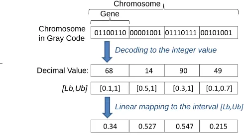
The algorithm uses a binary representation ofchromosomes as fixed-length strings over the alphabet{0,1}, such that they are well suited to handle the optimization problems. It uses function Encoding() to map solutions w~ ∈ W to a binary string {0,1}l and defines function Decoding() to do the reverse. To this end, real-valued vector w~ ∈ <n is presented
by a chromosome in form of a binary string ~x ∈ {0,1}l. The chromosome is logically divided into n segments (gene) of equal length Sgene as (w1...wn), where Sgene is gene
size and l = n×Sgene. Each gene wi is decoded to yield
the corresponding integer value, and the integer value is in turn linearly mapped to its interval of real values, denoted as [Lbi, U bi] ⊂ <, where Lbi and U bi indicate lower and
upper bound constraints on wi, respectively. In this work, we
use a gray code interpretation of the binary string. The main advantage of gray codes is that they are different by only one bit.
Figure 5 shows an example of the decoding process for string segments of length Sgene = 8 which allows the
rep-resentations of integers{0,1, ...,255}. As shown in the figure,
functionDecoding()first converts a given gray code to an in-teger valuepi∈
0, ...,2Sgene−1 and then mapsp
i linearly
to its corresponding intervalDecoding[Lbi, U bi]asLbi+2U bSgenei−Lb−i1×pi.
Ch
Gene
Chromosome
01100110 00001001 01110111 00101001
Chromosome in Gray Code
Decoding to the integer value
68 14 90 49
[0.1,1] [0.5,1] [0.3,1] [0.1,0.7] Decimal Value:
[Lb,Ub]
0.34 0.527 0.547 0.215 Linear mapping to the interval [Lb,Ub]
Fig. 5. An example of decoding and linear mapping
After encoding, the algorithm starts producing a new popula-tion in Line 5-20. Funcpopula-tionElitism()in Line 5 copies the best chromosome of the current population to the new population, so the best chromosome found can survive. Elitism can very rapidly increase performance of GA, because it prevents losing the best found solution. To create other new offsprings, three basic operators including selection, crossover, and mutation are applied as follows.
Selectionin GA means how to select parents for crossover or mutation. The main idea is to select the better parents in hope that the better parents will produce better offspring. Thus, functionSelection()in the algorithm selects randomly two chromosomes from the current population, evaluates their fitness values, and finally returns the one which has the smaller fitness value as one of parents. Another parent is selected in the same way.
Cross P rob in Line 8 is the crossover probability which states how often a crossover is performed. If there is a crossover, two parents’ chromosomes are selected and off-spring is made from their crossover. If there is no crossover, offspring is the exact copy of a chromosome from the old population. Due to Cross P rob, the new generation is a mix of offsprings made by crossovers and chromosomes from the old population. Although crossovers have the tendency to improve chromosomes, it has been shown to be beneficial to keep part of the old population.
Crossover selects genes from parents’ chromosomes and creates a new offspring. There are different ways to make a crossover. This algorithm chooses randomly two crossover points and everything before the first point and after the second point is copied from the first parent and the section between the two crossover points is copied from the second parent. Figure 6 shows an example of crossover applied in this algorithm (|
denotes the crossover point).
Crossover
Chromosome 1: 1011 101000 111010
Chromosome 2: 1100 101001 110011
Offspring: 1011101001 111010
Mutation
101110100011010 Offspring:
101010100111110 Mutated Offspring:
Fig. 6. An example of crossover
optimum. Mutation in Algorithm 3 changes the new offspring by randomly switching a few bits. It is worth mentioning that the mutation should not occur very often, because then GA will convert into a random search. Figure 7 shows an example of mutation used in the algorithm.
Crossover
1011 101000 111010
1100 101001 110011
Chromosome 1:
Chromosome 2:
1011101000111010
Offspring:
Mutation
Offspring: 1011101000111010
Mutated Offspring: 1010101001111110
Fig. 7. An example of mutation
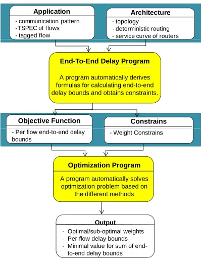
This process repeats for a specified number of iterations. As shown in Figure 8, we have developed a tool in C++, divided into two main sub-tools including End-to-End Delay Program andOptimization Program. The former derives per-flow worst-case bounds by applying the proposed formal approach in Section V. The bounds are represented as functions of weights in WRR policy. The latter optimizes weights in WRR policy based on the optimization problem formulated in Section VI. Input for the first sub-tool includes an application communication graph, specification of flows, topology graph, routing matrix, and characteristics of routers. The outputs from the first sub-tool along with the set of system constraints will be inputs for the second part. If flows or traffic pattern are changed, per-flow end-to-end delay bounds and optimization problem need to be resolved. Since we aim for a design phase tool, it is executed once for static flows.
IX. EXPERIMENTALRESULTS
To evaluate the potential of our method, we applied it to two real applications and a synthetic traffic pattern on a larger network.
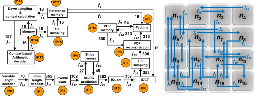
A. VOPD Application
We have applied our model to a real-time multimedia appli-cation with a random mapping to the tiles of a 4×4on-chip network. Figure 9 shows the task graph and flow mapping of a Video Object Plane Decoder (VOPD) [39] in which each block corresponds to an IP and the numbers near the edges represent the bandwidth (in MBytes/sec) of the data transfer, for a 30
frames/sec MPEG-4 movie with 1920×1088resolution [40]. There are 21 communication flows characterized by TSPEC.
Hence, each flow i is characterized by (Li, pi, σi, ρi). The
maximum transfer size and peak rate refer to the real traffic flow over the flit channel between routers. They are constrained by the flit channel capacity. Packets may have different burst sizes. They are sent flit by flit over the flit channel. This means the maximum transfer size of1f litand peak rate1f lit/cycle. Therefore, we assumeLiandpi for all flows are the same and
equal to1f litand1f lit/cycle, respectively.ρi is determined
Application
- communication pattern -TSPEC of flows - tagged flow
Architecture
- topology - deterministic routing - service curve of routers Input Text File
End-To-End Delay Program
A program automatically derives formulas for calculating end to end formulas for calculating end-to-end delay bounds and obtains constraints.
Output Text File Objective Function Constrains
Optimization Program
Output Text File
- Per flow end-to-end delay bounds
- Weight Constrains
A program automatically solves optimization problem based on
the different methods
Output - Optimal/sub-optimal weights - Per-flow delay bounds - Minimal value for sum of
end-to-end delay bounds
Fig. 8. The flow chart of the developed tool
in f lits/cycle due to associated bandwidth with flow fi in
Figure 9 and σi varies between8 and128 f lits for different
flows. The length of a round in WRR scheduling, LW R, is
assumed to be10cycles.
1) Delay Optimization: As mentioned before, decision vari-ables in the proposed optimization problems are the weights on shared channels. Due to shared channels in VOPD application,
20 weights are formulated in the optimizations as a weight vectorW defined as follows:
W = w(6,3,0,4), w(10,2,0,0), w(14,0,0,2), w(13,3,0,2), w(12,0,0,2),
w(9,4,0,0), w(4,3,0,4), w(4,0,0,2), w(8,2,0,0), w(8,4,0,2),
w(6,2,0,4), w(10,4,0,0), w(14,3,0,2), w(13,1,0,2), w(12,3,0,2),
w(9,3,0,0), w(4,0,0,4), w(4,4,0,2), w(8,4,0,0), w(8,0,0,2)
(16) The ”End-to-End Delay Program” calculates per-flow worst-case bounds as functions of weights for each flow in VOPD application and derives corresponding constraints. The ”Op-timization Program” formulates Minimize-Delay problem and derives weights for VOPD application.
To show how these weights affect the communication delay, we consider four different schemes:
• Random Scheme: The weights are selected randomly.
• Round Robin Scheme: The weights have the same values to represent round robin policy.
• Optimized Scheme: The weights are optimized based on the optimization problem (8).
Variable length decoder
70
Run-length decoder
362 Inverse
scan 362 predictionAC/DC 362 iQuant 357 IDCT Stripe
memory
49 27
Up sampling
VOP reconstruction
Padding VOP
memory
353 300 313 94
313 500
Context-based Arithmetic
decoder Memory Down sampling
& context calculation
157 16 16
Reference memory
Up sampling
16 16
16
16
16
1 f
2 f
3 f
5 f
4 f
6 f
8 f
7 f
9 f
10 f 11
f f12
13 f
14 f
15
f f16 f17
18
f f19
20
f f21
IP12 IP11
IP15 IP14
IP13
IP0 IP1 IP2 IP3 IP5 IP6
IP4 IP10
IP8
IP7
IP9
Fig. 9. VOPD Application
0 100 200 300 400 500 600 700 800 900
1 2 3 4 5 6 7 8 9 10 11 12 13 14 15 16 17 18 19 20 21
De
la
y
Bo
un
d
(c
yc
le
)
Flow Index
WRR Policy RR Policy
Fig. 10. Maximum worst-case delay for every flow in VOPD application
see that the optimized scheme leads to about 15.4%,48.8%, and81.1%reduction in total maximum delay when compared withRound Robin,Random, andUnoptimizedschemes, respec-tively. The results show that although WRR is able to make better performance in terms of latency than RR scheduling, if the weights are not allocated properly, it may be worse. Therefore, an appropriate weight configuration makes WRR able to reduce total and average maximum delay by balancing the allocation of shared network bandwidth to different traffic flows with respect to their specifications and contentions for shared resources.
To better understand the effects of the weights, per-flow delay bounds for RR and WRR with the Optimized scheme are shown in Fig 10. This figure illustrates that flows in WRR can experience longer or shorter delays than the RR scheme which depends on the amount of network bandwidth allocated to each flow (due to the assigned weights). However, from Table II, we can see that the total and average worst-case delay are decreased in WRR with theOptimizedscheme because the weights are assigned in a way to minimize total delay, satisfy performance constraints, and reduce contentions for shared resources leaving room for other contention interfering flows. Therefore, WRR can be used to control the per-flow delay bound by controlling its assigned weight.
It is worth mentioning that RR is a special case of WRR (all weights equal) and will most likely be found by the optimization algorithm when it is preferable according to the
0 100 200 300 400 500 600 700
1 2 3 4 5 6 7 8 9 10 11 12 13 14 15 16 17 18 19 20 21
Del
ay B
o
und
(c
yc
le)
Flow Index
Model
Simulation
Fig. 11. Comparison of delay bounds from the proposed model and simulator for VOPD application
defined optimization objectives.
We have investigated the accuracy of the proposed analytical model with the BookSim simulator in our previous work [4]. However, as we have extended the model to WRR policy, we compare per-flow delay bounds obtained from the analytical model and BookSim simulator [32] for theOptimizedscheme. The simulation uses the same assumptions as explained in [4]. As shown in Fig. 11, all delays observed in simulations are below the LUDB but not too far, suggesting that the analytical bound is fairly tight since the simulation typically does not exercise the worst case.
We have also computed the relative errors with respect to
TABLE II
HOWGOODAREOPTIMIZEDWEIGHTS?
Scheme Type Weight Vector
Total Worst-case Delay (cycles)
Average Worst-case Delay (cycles)
Optimized (2,8,8,2,6,6,4,2,3,6,
8,2,2,8,4,4,6,8,7,4) 3671 174
Round Robin (5,5,5,5,5,5,5,5,5,5,
5,5,5,5,5,5,5,5,5,5) 4237 202
Random (1,4,2,7,2,3,9,5,8,5, 9,6,8,3,8,7,1,5,2,5)
7177 343
Unoptimized (1,1,1,9,1,1,9,9,9,5, 9,9,9,1,9,9,1,1,1,5)
simulation results to consider the accuracy of the analytical model. The calculations show that the maximum and average relative errors are about 33.33%and16.3%, respectively.
Monitoring the delay of packets shows that worst-case delay is much larger than average-case delay, which is reasonable because worst-case bounds cover corner cases. We have also noticed that traffic burstiness has the most influence on the delay distribution. The larger the burstiness, the larger the delay variance.
2) Multi-objective Optimization: In the multi-objective op-timization minimizing delay and variance, we have calculated two parameters: Total Worst-case Delay and Variance listed in Table III. As can be observed from Table III, Minimize-Delay problem guarantees that weight allocation is carried out in favor of minimizing total worst-case delay while there is no such guarantee for the variance over various flows. In contrast, the Multi-objective optimization provides a trade-off between such parameters.
Under the Multi-objective optimization the standard devia-tion is less than 0.89 of the average delay because variance is an explicit target for minimization. It is also fairly small under the Minimize-Delay objective (standard deviation<1.1
of the average delay) because greater imbalances of flows (bigger variance) tend to lead to worse contention between flows and thus to higher average delays. Hence, the Minimize-Delay algorithm implicitly tends to reduce variance as well.
Although we have assumed the same importance for total delay and variance in the multi-objective problem by consid-ering the same weighting coefficients in Equation (15), it is possible for designers to change the value of the weighting coefficients γ1 and γ2 to specify another relative importance of objective functions.
3) Comparing with Other Solution Methods: As a compar-ative study, we implement three other metaheuristics, namely Pure Random Search (PRS) [33], Markov Monotonous Ap-proach (MMA)[34], andAdaptive Search (AS)[34] to compare them with the genetic algorithm in terms of run-time and effi-ciency. These algorithms belong to a category of metaheuristics called trajectory-based methods. A trajectory-based algorithm works on single solutions at any time, namely, it starts from an initial state (initial solution) and follows a trajectory to reach a successor solution which may or may not belong to the neighborhood of the current solution. Population-based metaheuristics, on the contrary, deal with a set (a population) of solutions in each iteration and in turn provide an intrinsic method for exploring the search space. The way of
manipulat-TABLE III
HOWGOOD ISMULTIOBJECTIVEOPTIMIZATION?
Weight Vector
Total Worst-case Delay (cycles)
Variance
Round Robin
(5,5,5,5,5,5,5,5,5,5,
5,5,5,5,5,5,5,5,5,5) 4237 59324.49
Minimize-Delay
(2,8,8,2,6,6,4,2,3,6,
8,2,2,8,4,4,6,8,7,4) 3671 35416.67
Multi-objective
(6,9,9,1,6,7,2,1,1,6
4,1,1,9,4,3,8,1,1,6) 4045 29320.71
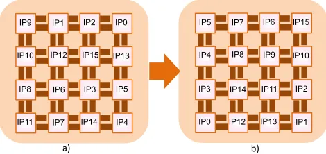
IP5 IP7 IP6 IP15
IP4 IP8 IP9 IP10
IP3 IP14 IP11 IP2
IP0 IP12 IP13 IP1 IP9 IP1 IP2 IP0
IP10 IP12 IP15 IP13
IP8 IP6 IP3 IP5
IP11 IP7 IP14 IP4
a) b)
Fig. 12. Two different mappings for VOPD application
ing the population has a significant impact on the performance of these methods. Genetic algorithms belong to this category. We also extend PRS, MMA, and AS to support a population of solutions instead of a single solution. Hereby, they produce m solutions in every iteration and select n solutions for the next iteration. The extended versions of PRS,MMA, and AS are called PRS (m+n), MMA (m+n), and AS (m+n). Table IV presents the iteration number and run time required for solving the optimization problem (Eq. 8).
The results show that all metaheuristics presented in this table obtain the same solution for the problem. Therefore, we can say with some confidence that the solution is of high quality.
The table shows that the genetic algorithm has a shorter execution time with fewer iterations. GA is no exhaustive optimization method. However, as it is well known that GAs provide an efficient and robust method for solving problems in which the objective function is discontinuous, nondifferen-tiable, or highly nonlinear and due to the results from table IV, we believe that GA is a well suited solution method for our problem.
4) Comparing with An Optimized Mapping: By this point, we have considered a random mapping for VOPD application as shown in Fig. 12a). To show how a good mapping affect the results from our approach, we take the optimized mapping shown in Fig. 12b) from PERMAP algorithm [42]. Table V presents Total Worst-case Delay parameter derived from our approach for different scenarios on these two mappings. As it can be seen, applying our technique along with a good mapping can give much better results in terms of delay minimization.
TABLE IV
COMPARISON OF THERUNTIME FORDIFFERENTMETHODS
Optimal point obtained by the methods
Optimal Weight Vector Total Delay
(2,8,8,2,6,6,4,2,3,6,8,2,2,8,4,4,6,8,7,4) 3671cycles
Performance in different methods
Iteration# Time(sec)
PRS 100,000 2.71
MMA 100,000 2.8
AS 100,000 2.85
PRS(10 + 10) 5,000 13 MMA(10 + 10) 5,000 13.37 AS(10 + 10) 5,000 12.83
5 0 1 2
6 7 10
11
12
13
15
16
17
18 20
21 22 23
24
3 4
8 9
14
19
H263 Encoder
MP3 Encoder MP3 Decoder
H263 Decoder
1
f
2
f
3
f
4
f f5 f6 f8 f7 f9 10
f
11
f
13
f
12
f f14
15
f
16
f
18
f
17
f
19
f
20
f
21
f
22
f
22
f
20 16
10 0 5
7 1 18
IP1 4
23
13 14
24
9
21 22 17 3 IP119
6 2 11 8 12
15
a) b)
Fig. 13. MMS Application
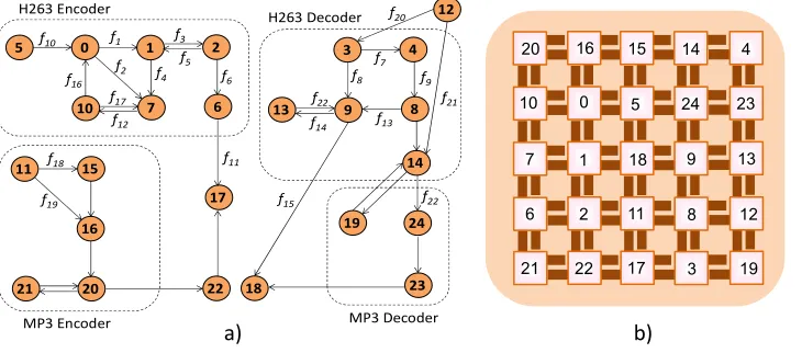
B. Mutlimedia Application
We have evaluated our method for a generic MultiMedia System (MMS). MMS is an integrated video/audio system which includes an H263 video encoder, an H263 video de-coder, an MP3 audio ende-coder, and an MP3 audio decoder. This application can be partitioned into 40 concurrent tasks and then these tasks are assigned onto 25 selected IPs [43]. These IPs range from DSPs, generic processors, and embedded DRAMs to customized application specific integrated circuits (ASICs). Real video and audio clips are used as inputs to derive the communication patterns among these IPs. Fig. 13a) reveals the communication task graph of this system [43]. We have applied the PERMAP algorithm [42] to get an optimized mapping for this system as shown in Fig. 13b).
Due to shared channels in the MMS application, weight vector W consisting of 37weights is defined as below:
W = w(16,1,0,0), w(15,3,0,2), w(15,0,0,2), w(5,3,0,0), w(14,4,0,2),
w(19,1,0,2), w(18,4,0,2), w(18,3,0,2), w(13,2,0,4), w(23,3,0,0),
w(14,1,0,4), w(10,2,0,4), w(1,0,0,4), w(1,3,0,4), w(11,4,0,0),
w(6,0,0,3), w(13,1,0,0), w(8,2,0,0), w(2,4,0,0), w(21,3,0,0),
w(16,4,0,0), w(15,4,0,2), w(5,4,0,0), w(14,0,0,2), w(19,4,0,2),
w(18,0,0,2), w(13,3,0,4), w(23,2,0,0), w(14,2,0,4), w(10,0,0,4),
w(1,1,0,4), w(11,2,0,0), w(6,1,0,3), w(13,4,0,0), w(8,4,0,0),
w(2,1,0,0), w(21,2,0,0)
(17) Fig. 14 depicts delay bounds for each flow under the RR policy and the optimized WRR scheme with Minimize-Delay. Although flows in WRR can experience longer or shorter delays than under the RR scheme, the optimized WRR scheme guarantees an appropriate weight allocation in terms
TABLE V
COMPARISON OFTOTALWORST-CASEDELAY WITH THERANDOM AND OPTIMIZEDMAPPINGS
Random Mapping PERMAP Mapping
Round Robin 4237 2385
Minimize-Delay 3671 2159
Multi-objective 4045 2544
Min Delay‐RR
Min Multi‐RR 0 100 200 300 400 500 600 700
1 2 3 4 5 6 7 8 9 10 11 12 13 14 15 16 17 18 19 20 21 22 23 24 25 26 27 28 29 30 31 32
Del
ay
B
o
und
(c
yc
le
)
Flow Index
WRR Policy
RR Policy
0 100 200 300 400 500 600 700
1 2 3 4 5 6 7 8 9 10 11 12 13 14 15 16 17 18 19 20 21 22 23 24 25 26 27 28 29 30 31 32
Del
ay
B
o
und
(c
yc
le
)
Flow Index
WRR Policy RR Policy
Fig. 14. Maximum worst-case delay for every flow in MMS application
of minimizing total worst-case delay.
For more detail, we have presented two parameters Total Worst-case DelayandVariancefor different defined scenarios in Table VI. As explained before, Minimize-Delay problem allocates weights such that guarantees total worst-case delay minimization and Multi-objective problem provide a trade-off between these two parameters.
TABLE VI
COMPARISONAMONGDIFFERENTSCENARIOS FORMMS APPLICATION
Weight Vector
Total Worst-case Delay (cycles)
Variance
Random Scheme
(5,4,4,7,9,3,1,1,9,9,7,4, 5,2,4,2,9,9,2,5,5,2,3,1,7 8,1,1,3,6,3,6,8,1,1,8,5)
13509 671014
Round Robin
(5,3,3,5,5,5,3,3,5,5,5,5, 3,3,5,5,5,5,5,5,5,4,5,5,5 4,5,5,5,5,4,5,5,5,5,5,5)
4783 26324.9
Minimize-Delay
(5,3,4,7,2,8,1,4,5,4,7,5, 5,2,4,2,1,4,2,5,5,3,3,8,2 5,5,6,3,5,3,6,8,9,6,8,5)
4034 14832.5
Multi-objective
(9,1,1,8,2,8,1,4,4,4,2,9, 1,1,1,5,1,1,6,1,1,8,2,8,2 5,6,6,8,1,8,9,5,9,9,4,9)
0 100 200 300 400 500 600 700 800 900 1000
1 3 5 7 9 11 13 15 17 19 21 23 25 27 29 31 33 35 37 39 41 43 45 47 49 51 53 55
D
e
la
y
Bo
u
n
d
(cycle
)
Flow Index WRR Policy RR Policy
Fig. 15. Maximum worst-case delay for every flow under transpose traffic pattern
C. Transpose Traffic Pattern
To investigate a larger network, we experiment a 8 ×8
mesh network under the transpose traffic pattern with 56 communication flows. The values of L and p are assumed
1 f lit and 1 f lit/cycle, respectively. For different flows, ρ varies between0.001 and0.03 f lits/cycle, andσbetween 2
and 128 f lits. Table VII presents the source and destination of flows along with the index assigned to them.
Similar to previous case studies, we depict per-flow worst-case delay bounds for RR policy and the optimized WRR scheme in Fig. 15. Regarding this figure, it is apparent that some flows in the optimized WRR policy may suffer longer delays than RR scheme. However, total delay bound in the optimized WRR scheme is equal to 17610 cycleswhile it is
19761 cycles in RR scheme. These values confirm that an appropriate weight allocation can guarantee total delay bound minimization in the network.
X. CONCLUSIONS
We have extended our earlier proposed methodology [4] for deriving per-flow delay bounds under RR policy to WRR scheduling and then compared them. We have developed algorithms to automate analysis steps. It is notable that the proposed methodologies for both RR and WRR do not deal with the back-pressure, but we have calculated the buffer size thresholds to make sure the back-pressure does not occur in the network. Based on these analytical models, we have presented two optimization problems for weight allocation in WRR scheduling, one for minimizing the total worst-case delays and one for minimizing both total worst-case delays and their vari-ance under performvari-ance requirements to control per-flow delay bounds. We have also demonstrated that the proposed model exerts significant impact on communication performance. The algorithm for solving the proposed minimization problems runs very fast. For the case study, the optimized solution is found within about one second. The contribution of this paper is providing a performance evaluation tool for designers to make a good decision at the design phase. The algorithm can be performed at run time as it is quite fast but it needs a control infrastructure to get feedback from the network and distribute the results. On the other hand modifying weights at run time is not easy. The way of applying the algorithm at run time can be considered as a future work. In the future, we intend to investigate other scheduling policies. We also plan to extend the proposed analytical method in case of
back-pressure in the network. Zhao and Lu [41] propose analytical models to derive worst-case bounds for constant bit rate flows due to back-pressure in the network. The current work does not consider speculative VC-allocation/switch allocation techniques. Extending the model to adjust these techniques can be considered as another future work. In this paper, we have assumed virtual-cut-through switching as the model is suitable for NoCs with small packets only. Small packet NoCs are a relevant and important, even in practice. Extension of the model to support wormhole routing is under our investigation. There are currently some papers in our group on wormhole routing but they consider only average behavior of flows [19] [44].
REFERENCES
[1] J. Y. L. Boudec and P. Thiran,”Network Calculus: A Theory of Determin-istic Queuing Systems for the Internet”, Number 2050 in LNCS, 2004. [2] F. Jafari, A. Jantsch, and Z. Lu, ”Output Process of Variable Bit-Rate
Flows in On-Chip Networks Based on Aggregate Scheduling”,in Proc. of the International Conference on Computer Design (ICCD), pp. 445-446, 2011.
[3] F. Jafari, A. Jantsch, Z. Lu, ”Worst-Case Delay Analysis of Variable Bit-Rate Flows in Network-on-Chip with Aggregate Scheduling”,in Proc. of Design, Automation and Test in Europe Conference (DATE), pp. 538-541, 2012.
[4] F. Jafari, Z. Lu, and A. Jantsch, ”Least Upper Delay Bound for VBR Flows in Networks-on-Chip with Virtual Channels”, ACM Transactions on Design Automation of Electronic Systems (TODAES), Vol. 20, No. 3, Article No. 35, June 2015.
[5] C. Blum and A. Roli, ”Metaheuristics in combinatorial optimization: Overview and conceptual comparison”,ACM Comput. Surv., Vol. 35, No. 3, pp. 268-308, 2003.
[6] A. E. Kiasari, A. E., Jantsch, A., and Z. Lu, Mathematical formalisms for performance evaluation of networks-on-chip, ACM Computing Surveys. Vol. 45, No. 3, Article No. 38, 2013.
[7] Y. Ben-Itzhak, I. Cidon, A. Kolodny, Average latency and link utilization analysis of heterogeneous wormhole NoCs,Integration, the VLSI Journal, Vol. 51, Issue C, pp. 92-106, 2015
[8] Qian et al. ”A Support Vector Regression (SVR) based Latency Model for Network-on-Chip (NoC) Architectures”,IEEE Transactions on CAD, Vol. PP, No. 99, pp. 1
[9] Qian et al. ”A comprehensive and accurate latency model for Network-on-Chip performance analysis,”in Proc. of Asia and South Pacific Design Automation Conference (ASP-DAC), pp. 323-328, 2014.
[10] Qian et al. ”SVR-NoC: a performance analysis tool for network-on-chips using learning-based support vector regression model”.In Proc. of Design, Automation and Test in Europe (DATE), pp. 354-357, 2013.
[11] P. Bogdan, M. Kas, R. Marculescu, O. Mutlu, ”QuaLe: A Quantum-Leap Inspired Model for Non-stationary Analysis of NoC Traffic in Chip Multi-processors”,in Proc. of the International Symposium on Networks-on-Chip (NOCS), pp. 241-248, 2010
TABLE VII
THE LIST OF FLOWS UNDER TRANSPOSE TRAFFIC PATTERN
f1: 0−→63 f15: 19−→37 f29: 63−→0 f43: 37−→19
f2: 1−→55 f16: 18−→45 f30: 55−→1 f44: 45−→18
f3: 2−→47 f17: 17−→53 f31: 47−→2 f45: 53−→17
f4: 3−→39 f18: 16−→61 f32: 39−→3 f46: 61−→16
f5: 4−→31 f19: 27−→36 f33: 31−→4 f47: 36−→27
f6: 5−→23 f20: 26−→44 f34: 23−→5 f48: 44−→26
f7: 6−→15 f21: 25−→52 f35: 15−→6 f49: 52−→25
f8: 13−→22 f22: 24−→60 f36: 22−→13 f50: 60−→24
f9: 12−→30 f23: 34−→43 f37: 30−→12 f51: 43−→34
f10: 11−→38 f24: 33−→51 f38: 38−→11 f52: 51−→33
f11: 20−→29 f25: 32−→59 f39: 29−→20 f53: 59−→32
f12: 10−→46 f26: 41−→50 f40: 46−→10 f54: 50−→41
f13: 9−→54 f27: 40−→58 f41: 54−→9 f55: 58−→40