Patron: Her Majesty The Queen Rothamsted Research Harpenden, Herts, AL5 2JQ
Telephone: +44 (0)1582 763133 Web: http://www.rothamsted.ac.uk/
Rothamsted Research is a Company Limited by Guarantee Registered Office: as above. Registered in England No. 2393175. Registered Charity No. 802038. VAT No. 197 4201 51. Founded in 1843 by John Bennet Lawes.
Rothamsted Repository Download
A - Papers appearing in refereed journals
Lu, B., Sun, H., Harris, P., Xu, M. and Charlton, M 2018. shp2graph: tools
to convert a spatial network into an igraph in R. ISPRS International
Journal of Geo-Information. 7 (8), p. 293.
The publisher's version can be accessed at:
•
https://dx.doi.org/10.3390/ijgi7080293
The output can be accessed at: https://repository.rothamsted.ac.uk/item/8489v.
© 24 July 2018. Licensed under the Creative Commons CC BY.
International Journal of
Geo-Information
Article
Shp2graph: Tools to Convert a Spatial Network into
an Igraph Graph in R
Binbin Lu1,2,*ID, Huabo Sun3, Paul Harris4, Miaozhong Xu2,*ID and Martin Charlton5 1 School of Remote Sensing and Information Engineering, Wuhan University, 129 Luoyu Road,
Wuhan 430079, China
2 State Key Laboratory of Information Engineering in Surveying, Mapping and Remote Sensing,
Wuhan University, 129 Luoyu Road, Wuhan 430079, China
3 Institute of Aviation Safety, China Academy of Civil Aviation Science and Technology, Beijing 100028, China;
4 Sustainable Agricultural Sciences, Rothamsted Research, North Wyke, Okehampton, Devon EX20 2SB, UK;
5 National Centre for Geocomputation, Maynooth University, Maynooth, County Kildare, Ireland;
* Correspondence: [email protected] (B.L.); [email protected] (M.X.); Tel.: +86-27-6877-0771 (B.L.); +86-27-6877-8032 (M.X.)
Received: 4 June 2018; Accepted: 19 July 2018; Published: 24 July 2018
Abstract:In this study, we introduce theRpackageshp2graph, which provides tools to convert a spatial network into an ‘igraph’ graph of theigraph Rpackage. This conversion greatly empowers a spatial network study, as the vast array of graph analytical tools provided inigraphare then readily available to the network analysis, together with the inherent advantages of being within theRstatistical computing environment and its vast array of statistical functions. Through three urban road network case studies, the calculation of road network distances withshp2graphand with igraphis demonstrated through four key stages: (i) confirming the connectivity of a spatial network; (ii) integrating points/locations with a network; (iii) converting a network into a graph; and (iv) calculating network distances (and travel times). Throughout, the requiredRcommands are given to provide a useful tutorial on the use ofshp2graph.
Keywords: Rsoftware;igraph; graph data model; network distance; network analysis
1. Introduction
The characterization of a spatial network such as a transportation network, a river or stream network or a social network with geo-tags/locations is important to many areas of spatial science such as those found in geography, ecology, agriculture and sociology [1]. Tools exist to achieve such a characterization, often contributing to a certain element, such as savings in computational overheads. This study bridges a particular gap in this tool set where a vector-format spatial network is converted to a graph model and in doing so, benefits from a rich resource of existing and useful graph-based analytical tools, all within theRstatistical computing environment. This conversion tool is provided in theRpackageshp2graph[2], where this study details its construction, properties and uses.
Generally, a spatial network is managed in a geospatial polyline vector format, where spatial entities are recorded as ‘spaghetti’ collections of 2D/3D geospatial coordinates [3]. This format benefits from the detailed geometrical properties of the spatial network in providing an accurate representation of the physical network. However, and following the observations made by Goodchild ([4], p. 401) “Data modelling is defined as the process discretizing spatial variation but may be confused with issues of data structure and driven by available software rather than by a concern for accurate representation.”
ISPRS Int. J. Geo-Inf.2018,7, 293 2 of 19
In this respect, this study’s aim of converting a spatial network model to a graph model provides more assurance and added value to any subsequent spatial analysis to the given network and associated data, together with a reduced computational burden. To conceptualize a spatial network model as a graph data model entails viewing the network as a set of nodes, occupying particular positions, that are joined in pairs by physical or ephemeral constructs [5]. In this manner, the graph data model represents the physical network with logical graph topologies, that is, a set of nodes joined together in pairs as edges. This structure enables computation along a network to benefit directly from graph theory [6] and the associated computational savings therein [7].
This research initially stemmed from a need to find shortest paths or calculate network distances for a set of locations and an associated spatial network, all within the R statistical computing environment [8], so that a local spatial regression model for hedonic house price could be directly calibrated using different distance metrics [9]. Here theRpackagegdistanceprovides routines to calculate least-cost distances and routes on geographic grids [10] but it is not applicable when a spatial network is in a vector format, for example, aSpatialLinesorSpatialLinesDataFrameobject in R[11]. For this, the only solution is to work outside ofRwith tools provided in ArcGIS [12], GRASS GIS [13], pgRouting [14] and OSMnx [15,16], say; or using packages such asNetworkX[17] and OSMnx[15] withinPython, a GIS protocol [18], OSM tools in spatialite[19] and Axwoman [20], say. This is of course problematic given the statistical functions and associated tools reside inR (e.g., for a local regression application, see [21,22]). Fortunately, theClibraryigraphprovides such a collection of network analysis tools and has an interface inR, that is, the igraphpackage [23] but where the computations have to be carried out with a special class of graphs in R, namely ‘igraph.’ Thus, to bridge this gap within theRenvironment, the packageshp2graphwas developed for converting a spatial network of vector format into an ‘igraph’ object, which is now presented in its entirety. Through this conversion, travel time distances, shortest paths and network distances can be calculated efficiently via a range of classic algorithms, including Dijkstra’s algorithm [24], Bellman–Ford’s algorithm [25,26] and Johnson’s algorithm [27].
This article is constructed in the following four sections. First, the basics of converting a spatial network to an ‘igraph’ graph are introduced. Secondly, the step by step procedure for calculating network distances withshp2graphandigraphis given. Thirdly, the same procedure is summarized and useful extensions are proposed. Finally, a summary is given together with suggestions for future spatial network tools.
2. Converting a Spatial Network into an ‘igraph’ Graph
2.1. The Graph Data Model
The graph data model plays a vital role in analyzing network structures. According to Beauquier, Berstel and Chrétienne in Mathis ([28], p xvi): “Graphs constitute the most widely used theoretical tool for the modelling and research of the properties of structured sets. They are employed each time we want to represent and study a set of connections (whether directed or not) between the elements of a finite set of objects.” From graph theory, a graph is generally constituted of two finite collections of vertices and edges (links between vertices), where its formulaic expression can be denoted as:
G= (V,E), whereV= {v1, ...,vn}is the set of vertices andE= vi,vj
vi,vj ∈V is the set of edges. Note the edges can be defined by a weighting functionw=
w vi,vj vi,vj
∈ E to qualify or quantify the relationships between vertices. Specifically, an edge isdirectedwhen it is attributed with an orientation. Conversely, it is anundirectededge if no orientation is clarified. A graph is called a directed graphif it containsdirectededges; otherwise, it is known as anundirected graph.
The graph data model provides a simplifying tool to define and represent a network structure with three types of relations:
ISPRS Int. J. Geo-Inf.2018,7, 293 3 of 19
(ii) vertex-edge relations, where the member-owner relationship is defined if it is a starting or ending vertex of an edge;
(iii) edge-edge relations, where the contiguity relationship between two edges is defined if they share one or more vertex.
A graph can be constructed with all these relations properly externalized. For a vector-format spatial network, it can be simply represented by a graph constituted by a set of vertices occupying particular positions in space and edges from physical connections [4]. In this sense, we can convert a spatial network into an ‘igraph’ graph in three steps:
Step 1. Extract objects from the spatial network as vertices and include an identifier (ID) and 2-D coordinate (x,y) for each vertex;
Step 2. Construct all the edges according to the vertex-vertex adjacency relationships and deliver them as an adjacency matrix or 2-D array;
Step 3. Use existing functions inigraphto create an ‘igraph’ graph.
These three steps can be conducted using theshp2graphfunctionsreadshpnwandnel2igraph where we provide examples in the following section.
2.2. Data Conversion
A vector-format spatial network is usually read as a SpatialLines or SpatialLinesDataFrame object in R, where each individual polyline is expressed as a set of coordinates connected sequentially [11]. Inshp2graph, the default input for graph conversion is assumed to be aSpatialLines orSpatialLinesDataFrameobject. The most straightforward conversion is to take all the endpoints or junctions as vertices, that is, obtaining the first and last locations of each polyline as the starting and ending vertices, respectively, of an edge in the converted graph. Observe that the endpoints from equivalent coordinates are regarded as a single vertex (i.e., a junction in the network); where the numerical precision of the coordinates may affect this conversion (i.e., a lower-level floating point definition may cause false junctions to be recognized). As an example, the following R code (snippet 1, withshp2graphloaded) converts a sampled part of the ‘Ontario road network’ (ORN) [29], as shown in Figure1a into an ‘igraph’ graph, as shown in Figure1b. Observe that the coordinates of the vertices have been incorporated autonomously as vertex attributes “x” and “y.”
Code snippet 1:
data(ORN) plot(ORN.nt)
title(“The ORN spatial network”) rtNEL1 <-readshpnw(ORN.nt)
igr1 <-nel2igraph(rtNEL1[[2]], rtNEL1[[3]])
plot(igr1, vertex.label = NA, vertex.size = 2, vertex.size2 = 2, mark.col = “green”, main = “The converted igraph graph”)
summary(igr1)
IGRAPH U- 298 343 --+ attr: x (v/n), y (v/n)
ISPRS Int. J. Geo-Inf.2018,7, 293 4 of 19
that is, 298 and 343, respectively. Observe that the parameterea.propis used here to denote whether the attributes of each polyline should be kept for the edges.
Code snippet 2:
rtNEL2 <-readshpnw(ORN.nt, Detailed = TRUE, ea.prop = rep(0, 37)) igr2 <-nel2igraph(rtNEL2[[2]], rtNEL2[[3]])
plot(igr2, vertex.label = NA, vertex.size = 1, vertex.size2 = 1, main = “The converted
igraph graph with all the geometric properties”) summary(igr2)
IGRAPH U- 597 642 --+ attr: x (v/n), y (v/n)
ISPRS Int. J. Geo‐Inf. 2018, 7, x FOR PEER REVIEW 4 of 18
Code snippet 2:
rtNEL2 <‐readshpnw(ORN.nt, Detailed = TRUE, ea.prop = rep(0, 37)) igr2 <‐nel2igraph(rtNEL2[[2]], rtNEL2[[3]])
plot(igr2, vertex.label = NA, vertex.size = 1, vertex.size2 = 1, main = “The converted igraph graph with all the geometric properties”)
summary(igr2)
IGRAPH U‐‐‐ 597 642 ‐‐ + attr: x (v/n), y (v/n)
(a) (b)
Figure 1. Network to graph conversion by taking all the endpoints or junctions as vertices (Ontario
road data). (a) The ORN spatial network, (b) The resultant ‘igraph’ graph.
Figure 2. The converted ‘igraph’ graph with all geometric properties retained (Ontario road data).
Thus, we have provided two strategies for converting a spatial network into an ‘igraph’ object
and the desired network‐based analysis can follow accordingly, where it is enhanced by having the
many useful functions and algorithms in igraph now readily available. For example, we can calculate
network distances or shortest paths with shp2graph and igraph in R and this process is detailed
below. Furthermore, shp2graph can easily be extended to different conversion strategies. For
example, taking complex objects as vertices (see master_node definition in [30]), or taking polylines
Figure 1.Network to graph conversion by taking all the endpoints or junctions as vertices (Ontario
road data). (a) The ORN spatial network, (b) The resultant ‘igraph’ graph.
ISPRS Int. J. Geo‐Inf. 2018, 7, x FOR PEER REVIEW 4 of 18
Code snippet 2:
rtNEL2 <‐readshpnw(ORN.nt, Detailed = TRUE, ea.prop = rep(0, 37)) igr2 <‐nel2igraph(rtNEL2[[2]], rtNEL2[[3]])
plot(igr2, vertex.label = NA, vertex.size = 1, vertex.size2 = 1, main = “The converted igraph graph with all the geometric properties”)
summary(igr2)
IGRAPH U‐‐‐ 597 642 ‐‐ + attr: x (v/n), y (v/n)
(a) (b)
Figure 1. Network to graph conversion by taking all the endpoints or junctions as vertices (Ontario
road data). (a) The ORN spatial network, (b) The resultant ‘igraph’ graph.
Figure 2. The converted ‘igraph’ graph with all geometric properties retained (Ontario road data).
Thus, we have provided two strategies for converting a spatial network into an ‘igraph’ object
and the desired network‐based analysis can follow accordingly, where it is enhanced by having the
many useful functions and algorithms in igraph now readily available. For example, we can calculate
network distances or shortest paths with shp2graph and igraph in R and this process is detailed
below. Furthermore, shp2graph can easily be extended to different conversion strategies. For
example, taking complex objects as vertices (see master_node definition in [30]), or taking polylines
ISPRS Int. J. Geo-Inf.2018,7, 293 5 of 19
Thus, we have provided two strategies for converting a spatial network into an ‘igraph’ object and the desired network-basedanalysis can follow accordingly, where it is enhanced by having the many useful functions and algorithms inigraphnow readily available. For example, we can calculate network distances or shortest paths withshp2graphandigraphinRand this process is detailed below. Furthermore,shp2graphcan easily be extended to different conversion strategies. For example, taking complex objects as vertices (see master_node definition in [30]), or taking polylines themselves as vertices for conversion to a connectivity graph [31]. Note that this conversion would assume planarity in the produced ‘igraph’ object (see similar conversions defined in [32]), which is largely dependent on the data structure of the original spatial network (like 2-D coordinates), or models with them. However, overpasses (viaducts) and underpasses (tunnels) in an urban road network bring typical nonplanarity [33], which can only be properly treated here by ensuring topological correctness at overpasses or underpasses, that is, no intersections.
3. Calculating Network Distances with Shp2graph and Igraph
Thedevelopmentofshp2graphwas motivated by the need to provide solutions to the calculation of network distances and shortest paths within theRstatistical computing environment. Theshp2graph Rpackage provides routines to convert a vector-format spatial network into an ‘igraph’ graph, allowing functions such asdistances,distance_table,shortest_pathsandall_shortest_pathsin theigraph Rpackage to be utilized. In practice, however, the conversions are rarely straightforward, where extra pre-processing operations are often required—such as checking the topology, optimizing the network structure and so forth.
As a case study to demonstrate the calculation of network distance (and travel time) matrices, we use the same London house price data (as provided by the Nationwide Building Society of the United Kingdom) and the same London road network (as produced by the UK Ordnance Survey (OS) in 2001), as that used in the local regression study of Lu et al. [9]. These example data sets are both available the latest release ofshp2graph. Thus, if the following R code is run (snippet 3), then the map of Figure3 results, where both data sets are combined.
Code snippet 3:
require(RColorBrewer) data(LNNT)
data(LNHP)
road.type <- unique(LN.nt$nt_RoadTyp) idx <- match(LN.nt$nt_RoadTyp, road.type) ltypes <- c(1, 1, 3, 1)
lwidths <- c(1, 1.5, 0.2, 2) shades <- brewer.pal(4, “Dark2”)
plot(LN.nt, col = shades[idx], lty = ltypes[idx], lwd = lwidths[idx], cex = 0.3) points(coordinates(LN.prop), pch = 15)
ISPRS Int. J. Geo-Inf.2018,7, 293 6 of 19
ISPRS Int. J. Geo‐Inf. 2018, 7, x FOR PEER REVIEW 5 of 18
themselves as vertices for conversion to a connectivity graph [31]. Note that this conversion would
assume planarity in the produced ‘igraph’ object (see similar conversions defined in [32]), which is
largely dependent on the data structure of the original spatial network (like 2‐D coordinates), or
models with them. However, overpasses (viaducts) and underpasses (tunnels) in an urban road
network bring typical nonplanarity [33], which can only be properly treated here by ensuring
topological correctness at overpasses or underpasses, that is, no intersections.
3. Calculating Network Distances with Shp2graph and Igraph
The development of shp2graph was motivated by the need to provide solutions to the calculation
of network distances and shortest paths within the R statistical computing environment. The
shp2graph R package provides routines to convert a vector‐format spatial network into an ‘igraph’
graph, allowing functions such as distances, distance_table, shortest_paths and all_shortest_paths in the
igraph R package to be utilized. In practice, however, the conversions are rarely straightforward,
where extra pre‐processing operations are often required—such as checking the topology, optimizing
the network structure and so forth.
As a case study to demonstrate the calculation of network distance (and travel time) matrices,
we use the same London house price data (as provided by the Nationwide Building Society of the
United Kingdom) and the same London road network (as produced by the UK Ordnance Survey (OS)
in 2001), as that used in the local regression study of Lu et al. [9]. These example data sets are both
available the latest release of shp2graph. Thus, if the following R code is run (snippet 3), then the
map of Figure 3 results, where both data sets are combined.
Code snippet 3:
require(RColorBrewer) data(LNNT)
data(LNHP)
road.type <‐ unique(LN.nt$nt_RoadTyp) idx <‐ match(LN.nt$nt_RoadTyp, road.type) ltypes <‐ c(1, 1, 3, 1)
lwidths <‐ c(1, 1.5, 0.2, 2)
shades <‐ brewer.pal(4, “Dark2”)
plot(LN.nt, col = shades[idx], lty = ltypes[idx], lwd = lwidths[idx], cex = 0.3) points(coordinates(LN.prop), pch = 15)
legend(551000, 172000, legend = road.type, lty = ltypes, lwd = lwidths, col = shades, title = “Road type”)
Figure 3. Case study data sets: London house price and road network data.
Figure 3.Case study data sets: London house price and road network data.
3.1. Confirming Connectivity in a Spatial Network
Completeness and topology correctness are fundamental for ensuring connectivity in a spatial network [34]. Whether or not a spatial network is self-connected, where no disconnected portions or islands exist in the network, that is, at least one path could be found between any pair of vertices. Connectivity is essential for calculating network distances or shortest paths successfully. To confirm the connectivity of a given spatial network theshp2graphfunction,nt.connect, searches through all the self-connected parts in the input network and returns a series of self-connected parts with the most vertices. In this sense, it always possible to get at least one self-connected network from this output. We can demonstrate this function as follows with thisRcode (snippet 4) together with the mapped output in Figure4:
Code snippet 4:
LN.nt.con <- nt.connect(LN.nt) plot(LN.nt.con)
ISPRS Int. J. Geo‐Inf. 2018, 7, x FOR PEER REVIEW 6 of 18
3.1. Confirming Connectivity in a Spatial Network
Completeness and topology correctness are fundamental for ensuring connectivity in a spatial
network [34]. Whether or not a spatial network is self‐connected, where no disconnected portions or
islands exist in the network, that is, at least one path could be found between any pair of vertices.
Connectivity is essential for calculating network distances or shortest paths successfully. To confirm
the connectivity of a given spatial network the shp2graph function, nt.connect, searches through all
the self‐connected parts in the input network and returns a series of self‐connected parts with the
most vertices. In this sense, it always possible to get at least one self‐connected network from this
output. We can demonstrate this function as follows with this R code (snippet 4) together with the
mapped output in Figure 4:
Code snippet 4:
LN.nt.con <‐ nt.connect(LN.nt) plot(LN.nt.con)
Figure 4. Connectivity of the London road network data via the function nt.connect.
Figure 4 clearly indicates that the London road network is highly self‐connected, where only one
self‐connected part was found (the plot title always returns this). This level of connectivity is
sufficient for subsequent operations and analyses and is expected for a carefully prepared network
data set. In practice, however, many spatial network data sets have poor connectivity conditions,
requiring much pre‐processing. In this respect, it is useful to provide another example—this time
using part of the Estevan road network downloaded from OpenStreetMap [35]. Thus, the following
R commands (snippet 5) returns this network’s connectivity conditions (mapped in Figure 5):
Code snippet 5:
data(ERN_OSM)
ERN.con <‐ nt.connect(ERN_OSM.nt) plot(ERN.con)
ISPRS Int. J. Geo-Inf.2018,7, 293 7 of 19
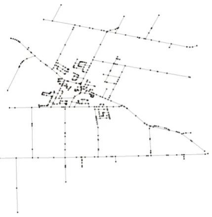
Figure4clearly indicates that the London road network is highly self-connected, where only one self-connected part was found (the plot title always returns this). This level of connectivity is sufficient for subsequent operations and analyses and is expected for a carefully prepared network data set. In practice, however, many spatial network data sets have poor connectivity conditions, requiring much pre-processing. In this respect, it is useful to provide another example—this time using part of the Estevan road network downloaded from OpenStreetMap [35]. Thus, the following R commands (snippet 5) returns this network’s connectivity conditions (mapped in Figure5):
Code snippet 5:
data(ERN_OSM)
ERN.con <- nt.connect(ERN_OSM.nt) plot(ERN.con)
ISPRS Int. J. Geo‐Inf. 2018, 7, x FOR PEER REVIEW 7 of 18
Figure 5. Connectivity of the Estevan road network via the function nt.connect.
As shown in Figure 5, the Estevan road network is comprised of ten unconnected parts marked
in ten different colors. Such poor connectivity is likely due to various topology errors, where the three
most common types are: dangling arc, overshoot and undershoot [36]. These are illustrated in Figure
6a–c and are defined as follows:
Dangling arc (Figure 6a): an arc featured by having the same polygon on both its sides and at
least one vertex that does not connect to any other arc, which is especially harmful for the
connectivity of the converted graph when both nodes are not connected to any other arc;
Overshoot (Figure 6b): an arc passes another arc which should intersect and stop there;
Undershoot (Figure 6c): an arc does not extend long enough to another arc which it should intersect.
(a) (b)
(c)
Figure 6. Three common types of topology errors. (a) Dangling arc, (b) Undershoot, (c) Overshoot.
Such topology errors lead to critical connectivity problems for the converted igraph graph and
as a consequence, cause failures in calculating shortest paths or network distances. Using the function
Figure 5.Connectivity of the Estevan road network via the functionnt.connect.
As shown in Figure5, the Estevan road network is comprised of ten unconnected parts marked in ten different colors. Such poor connectivity is likely due to various topology errors, where the three most common types are: dangling arc, overshoot and undershoot [36]. These are illustrated in Figure6a–c and are defined as follows:
Dangling arc (Figure6a): an arc featured by having the same polygon on both its sides and at least one vertex that does not connect to any other arc, which is especially harmful for the connectivity of the converted graph when both nodes are not connected to any other arc;
Overshoot (Figure6b): an arc passes another arc which should intersect and stop there;
ISPRS Int. J. Geo-Inf.2018,7, 293 8 of 19
ISPRS Int. J. Geo‐Inf. 2018, 7, x FOR PEER REVIEW 7 of 18
Figure 5. Connectivity of the Estevan road network via the function nt.connect.
As shown in Figure 5, the Estevan road network is comprised of ten unconnected parts marked
in ten different colors. Such poor connectivity is likely due to various topology errors, where the three
most common types are: dangling arc, overshoot and undershoot [36]. These are illustrated in Figure
6a–c and are defined as follows:
Dangling arc (Figure 6a): an arc featured by having the same polygon on both its sides and at
least one vertex that does not connect to any other arc, which is especially harmful for the
connectivity of the converted graph when both nodes are not connected to any other arc;
Overshoot (Figure 6b): an arc passes another arc which should intersect and stop there;
Undershoot (Figure 6c): an arc does not extend long enough to another arc which it should intersect.
(a) (b)
(c)
Figure 6. Three common types of topology errors. (a) Dangling arc, (b) Undershoot, (c) Overshoot.
Such topology errors lead to critical connectivity problems for the converted igraph graph and
as a consequence, cause failures in calculating shortest paths or network distances. Using the function
Figure 6.Three common types of topology errors. (a) Dangling arc, (b) Undershoot, (c) Overshoot.
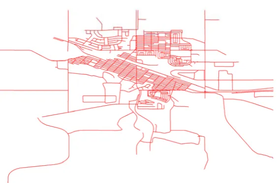
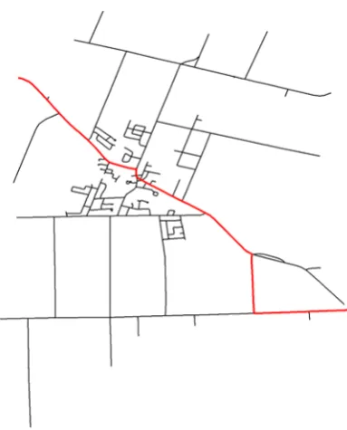
Such topology errors lead to critical connectivity problems for the convertedigraphgraph and as a consequence, cause failures in calculating shortest paths or network distances. Using the function nt.connectallows the user to find the main self-connected part, where all remaining unconnected parts can be dropped and thus provides an immediate solution for finding a self-connected network. However, this dropping of network parts is not always acceptable, especially when the dropped (unconnected) parts are clearly important to understanding the spatial process. This is the case for the Estevan road network example, where the main self-connected part (as shown in Figure7), aSpatialLinesDataFrameobjectERN.conreturned bynt.connect, does not adequately cover the study area (see the red part in Figure6). In this instance, we have to move outside of R, where there are a number of GIS tools available to correct topology errors, for example, topology error fixes in ArcGIS [37], polyline tools in ET Geo-tools [37] and a toolset for cleaning topology in GRASS [13]. In this instance, we processed the Estevan road data with the GRASS tools and got a new network with all topology errors fixed. The topology corrected data has been incorporated intoshp2graph, as demonstrated by the following R commands (snippet 6) and mapped in Figure8:
Code snippet 6:
data(ERN_OSM_correct)
ISPRS Int. J. Geo-Inf.2018,7, 293 9 of 19
ISPRS Int. J. Geo‐Inf. 2018, 7, x FOR PEER REVIEW 8 of 18
nt.connect allows the user to find the main self‐connected part, where all remaining unconnected parts
can be dropped and thus provides an immediate solution for finding a self‐connected network.
However, this dropping of network parts is not always acceptable, especially when the dropped
(unconnected) parts are clearly important to understanding the spatial process. This is the case for
the Estevan road network example, where the main self‐connected part (as shown in Figure 7), a
SpatialLinesDataFrame object ERN.con returned by nt.connect, does not adequately cover the study area
(see the red part in Figure 6). In this instance, we have to move outside of R, where there are a number
of GIS tools available to correct topology errors, for example, topology error fixes in ArcGIS [37],
polyline tools in ET Geo‐tools [37] and a toolset for cleaning topology in GRASS [13]. In this instance,
we processed the Estevan road data with the GRASS tools and got a new network with all topology
errors fixed. The topology corrected data has been incorporated into shp2graph, as demonstrated by
the following R commands (snippet 6) and mapped in Figure 8:
Code snippet 6:
data(ERN_OSM_correct)
ERN_cor.con <‐ nt.connect(ERN_OSM_cor.nt)
Figure 7. The main self‐connected part of the Estevan road network returned by the function nt.connect.
Figure 8. Connectivity of the Estevan road network with topology errors fixed via the function nt.connect.
In summary, it is important to confirm the connectivity of a given spatial network, which can be
achieved via the function nt.connect, supported by external GIS tools. Clearly, the incorporation of
such GIS tools within R would be a useful advance, further avoiding troublesome data imports and
exports that shp2graph goes some way in addressing. Note however, that these tools can themselves
create new topology errors. For example, when a bridge crosses over a road (or multiple bridges/roads,
as in the U.S. Interstate System), resulting in incorrect splits and the creation of false junctions.
Figure 7.The main self-connected part of the Estevan road network returned by the functionnt.connect.
ISPRS Int. J. Geo‐Inf. 2018, 7, x FOR PEER REVIEW 8 of 18
nt.connect allows the user to find the main self‐connected part, where all remaining unconnected parts
can be dropped and thus provides an immediate solution for finding a self‐connected network.
However, this dropping of network parts is not always acceptable, especially when the dropped
(unconnected) parts are clearly important to understanding the spatial process. This is the case for
the Estevan road network example, where the main self‐connected part (as shown in Figure 7), a
SpatialLinesDataFrame object ERN.con returned by nt.connect, does not adequately cover the study area
(see the red part in Figure 6). In this instance, we have to move outside of R, where there are a number
of GIS tools available to correct topology errors, for example, topology error fixes in ArcGIS [37],
polyline tools in ET Geo‐tools [37] and a toolset for cleaning topology in GRASS [13]. In this instance,
we processed the Estevan road data with the GRASS tools and got a new network with all topology
errors fixed. The topology corrected data has been incorporated into shp2graph, as demonstrated by
the following R commands (snippet 6) and mapped in Figure 8:
Code snippet 6:
data(ERN_OSM_correct)
ERN_cor.con <‐ nt.connect(ERN_OSM_cor.nt)
Figure 7. The main self‐connected part of the Estevan road network returned by the function nt.connect.
Figure 8. Connectivity of the Estevan road network with topology errors fixed via the function nt.connect.
In summary, it is important to confirm the connectivity of a given spatial network, which can be
achieved via the function nt.connect, supported by external GIS tools. Clearly, the incorporation of
such GIS tools within R would be a useful advance, further avoiding troublesome data imports and
exports that shp2graph goes some way in addressing. Note however, that these tools can themselves
create new topology errors. For example, when a bridge crosses over a road (or multiple bridges/roads,
as in the U.S. Interstate System), resulting in incorrect splits and the creation of false junctions.
Figure 8. Connectivity of the Estevan road network with topology errors fixed via the function
nt.connect.
In summary, it is important to confirm the connectivity of a given spatial network, which can be achieved via the functionnt.connect, supported by external GIS tools. Clearly, the incorporation of such GIS tools within R would be a useful advance, further avoiding troublesome data imports and exports thatshp2graphgoes some way in addressing. Note however, that these tools can themselves create new topology errors. For example, when a bridge crosses over a road (or multiple bridges/roads, as in the U.S. Interstate System), resulting in incorrect splits and the creation of false junctions.
3.2. Integrating Points with a Spatial Network
ISPRS Int. J. Geo-Inf.2018,7, 293 10 of 19
or (3) adding a pseudo edge to connect each point with its nearest vertex; or (4) adding a pseudo edge to connect each point with its nearest geometric point. These four strategies are illustrated in Figure9.
As illustrated in Figure9a, the most straightforward way (strategy 1) is to associate each pointPti
with its nearest vertex within the network, where this strategy rule is expressed as follows:
Pti(xi,yi)←arg min v∈V(g)
dist(Pti,v) =
q
(xi−xv)2+ (yi−yv)2
(1)
where(xi,yi)are the coordinates for the point/location Pti andvis a vertex of the graph gto be
converted with the coordinates(xv,yv). The nearest vertex is used to representPti, as marked with a
red circle in Figure9a. Strategy 1 is simple and computationally efficient but can be inaccurate when the network is sparse, or when only the endpoints of each polyline are recognized as vertices.
To get more accurate results than that found in strategy 1, strategy 2 finds the nearest geometric position on the network for each pointPtiand takes that position as a vertex (maybe newly added or
not) for representation. Thus, strategy 2 searches for the minimum distance between the pointPtiand
all the line segments and then fixes the nearest position as a representative vertex. This strategy rule is expressed as follows:
Pti(xi,yi)←Vposmin∈LSmin
←arg min
LS∈SN
dist(Pti,LS) =
|(y2−y1√)xi−(x2−x1)yi+(y1x2−y2x1)|
(y2−y1)2+(x2−x1)2
, x⊥∈range(x1,x2)&
y⊥∈range(y1,y2)
min
dj
dj=
q
(yi−yi)2+ xj−xi
2 ,i=1, 2
, otherwise (2)
where(x1,y1)and(x2,y2)are the coordinates of two endpoints of any line segmentLSin the network; posmin is the nearest position on the closest line segment LSmin and taken as the (new) vertex to represent the pointPti ;(x⊥,y⊥)are the coordinates of the foot point fromPti to the straight line
where the segmentLSis located and are found as follows:
x⊥= (x2−x1)
2x
i+(y2−y1)(x2−x1)yi−(y2−y1)(y1x2−y2x1) (y2−y1)2+(x2−x1)2
y⊥= (y2−y1)(x2−x1)xi+(y2−y1)
2y
i+(x2−x1)(y1x2−y2x1) (y2−y1)2+(x2−x1)2
(3)
Strategies 1 and 2 take typical vertices from the original spatial network to provide a virtual representation of the given points/locations. However, they can be deficient in that a certain loss of information is likely, particularly when the network is sparse, or there are comparatively large gaps between the network and points. In this respect, two further strategies 3 and 4 are available in the functionpoints2networkthat add pseudo edges between the given points and typical vertices are selected accordingly, as shown in Figure9c,d. This way, the points/locations themselves can be recognized as vertices. Note however, that the pseudo edges created by strategies 3 and 4 do not have homologous attributes as the original ones in the network, which may result in difficulties in a subsequent analysis.
ISPRS Int. J. Geo-Inf.2018,7, 293 11 of 19
ISPRS Int. J. Geo‐Inf. 2018, 7, x FOR PEER REVIEW 10 of 18
Strategies 1 and 2 take typical vertices from the original spatial network to provide a virtual
representation of the given points/locations. However, they can be deficient in that a certain loss of
information is likely, particularly when the network is sparse, or there are comparatively large gaps
between the network and points. In this respect, two further strategies 3 and 4 are available in the
function points2network that add pseudo edges between the given points and typical vertices are
selected accordingly, as shown in Figure 9c,d. This way, the points/locations themselves can be
recognized as vertices. Note however, that the pseudo edges created by strategies 3 and 4 do not have
homologous attributes as the original ones in the network, which may result in difficulties in a
subsequent analysis.
As demonstration, the following R commands (snippet 7) can be run for the Ontario road data,
resulting in the network maps presented in Figure 10a–d, where the function ptsinnt.view visualizes
the output from points2network. A list of vertices and the corresponding vertex‐vertex adjacency
matrix are returned by points2network, in preparation for subsequent conversion and associated
computations (this list can be particularly important for assessing the consequences of point
integration strategies 3 and 4). From Figure 10, observe that only the endpoints of the polylines are
viewed as vertices, which is a default option of the function points2network. All the geometric points
of each polyline are viewed as vertices if the parameter ‘Detailed’ in points2network is set as TRUE,
where accuracy can improve when point integration strategies 1 or 3 are adopted. This setting should
not be used for strategies 2 or 4 as outcomes are meaningless.
(a) (b)
(c) (d)
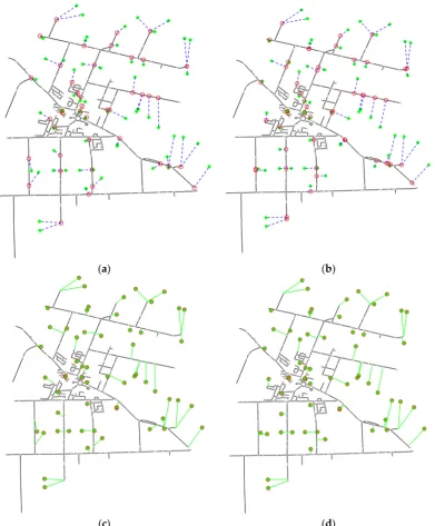
Figure 9. Four strategies to integrate points/locations within the spatial network. (a) Strategy 1:
represent each point with its nearest vertex; (b) Strategy 2: represent each point with its nearest
geometric point; (c) Strategy 3: add a pseudo edge (colored green) between each point and its nearest
vertex; (d) Strategy 4: Add a pseudo edge (colored green) between each point and its nearest
geometric point.
Code snippet 7:
data(ORN)
pts <‐ spsample(ORN.nt, 100, type = “random”) ptsxy <‐ coordinates(pts)[, 1:2]
ptsxy <‐ cbind(ptsxy[, 1] + 0.008, ptsxy[, 2] + 0.008)
res.nv <‐ points2network(ntdata = ORN.nt, pointsxy = ptsxy, ELComputed = TRUE, approach = 1) ptsinnt.view(ntdata = ORN.nt, nodelist = res.nv[[1]], pointsxy = ptsxy, CoorespondIDs = res.nv[[3]]) res.np <‐ points2network(ntdata = ORN.nt, pointsxy = ptsxy, approach = 2, ea.prop = rep(0, 2))
Figure 9. Four strategies to integrate points/locations within the spatial network. (a) Strategy 1:
represent each point with its nearest vertex; (b) Strategy 2: represent each point with its nearest geometric point; (c) Strategy 3: add a pseudo edge (colored green) between each point and its nearest vertex; (d) Strategy 4: Add a pseudo edge (colored green) between each point and its nearest geometric point.
Code snippet 7:
data(ORN)
pts <- spsample(ORN.nt, 100, type = “random”) ptsxy <- coordinates(pts)[, 1:2]
ptsxy <- cbind(ptsxy[, 1] + 0.008, ptsxy[, 2] + 0.008)
res.nv <- points2network(ntdata = ORN.nt, pointsxy = ptsxy, ELComputed = TRUE, approach = 1)
ptsinnt.view(ntdata = ORN.nt, nodelist = res.nv[[1]], pointsxy = ptsxy, CoorespondIDs = res.nv[[3]])
res.np <- points2network(ntdata = ORN.nt, pointsxy = ptsxy, approach = 2, ea.prop = rep(0, 2))
ptsinnt.view(ntdata = ORN.nt, nodelist = res.np[[1]], pointsxy = ptsxy, LComputed = TRUE, CoorespondIDs = res.np[[3]])
res.vnv <- points2network(ntdata = ORN.nt, pointsxy = ptsxy, ELComputed = TRUE, approach = 3, ea.prop = rep(0, 2))
ptsinnt.view(ntdata = ORN.nt, nodelist = res.vnv[[1]], pointsxy = ptsxy, CoorespondIDs = res.vnv[[3]], VElist = res.vnn[[7]])
res.vnp <- points2network(ntdata = ORN.nt, pointsxy = ptsxy, ELComputed = TRUE, approach = 4, ea.prop = rep(0, 2))
ISPRS Int. J. Geo-Inf.2018,7, 293 12 of 19
ISPRS Int. J. Geo‐Inf. 2018, 7, x FOR PEER REVIEW 11 of 18
ptsinnt.view(ntdata = ORN.nt, nodelist = res.np[[1]], pointsxy = ptsxy, ELComputed = TRUE, CoorespondIDs = res.np[[3]])
res.vnv <‐ points2network(ntdata = ORN.nt, pointsxy = ptsxy, ELComputed = TRUE, approach = 3, ea.prop = rep(0, 2))
ptsinnt.view(ntdata = ORN.nt, nodelist = res.vnv[[1]], pointsxy = ptsxy, CoorespondIDs = res.vnv[[3]], VElist = res.vnn[[7]])
res.vnp <‐ points2network(ntdata = ORN.nt, pointsxy = ptsxy, ELComputed = TRUE, approach = 4, ea.prop = rep(0, 2))
ptsinnt.view(ntdata = ORN.nt, nodelist = res.vnp[[1]], pointsxy = ptsxy, CoorespondIDs = res.vnp[[3]], VElist = res.vnp[[7]])
(a) (b)
(c) (d)
Figure 10. Examples of integrating points/locations with a spatial network (Ontario road data), where
green dots represent points given, a blue dash in (a,b) indicate the closest relationship between a point
and its nearest vertex/position on the network, green lines in (c,d) mean the edges newly added and
red circles mark the representative vertices. (a) Solution with strategy 1; (b) Solution with strategy 2;
(c) Solution with strategy 3; (d) Solution with strategy 4.
Figure 10.Examples of integrating points/locations with a spatial network (Ontario road data), where
green dots represent points given, a blue dash in (a,b) indicate the closest relationship between a point and its nearest vertex/position on the network, green lines in (c,d) mean the edges newly added and red circles mark the representative vertices. (a) Solution with strategy 1; (b) Solution with strategy 2; (c) Solution with strategy 3; (d) Solution with strategy 4.
ISPRS Int. J. Geo-Inf.2018,7, 293 13 of 19
improved by establishing a spatial index of the network, like using a boundary box to roughly track each road segment. This is a subject of on-going work.
ISPRS Int. J. Geo‐Inf. 2018, 7, x FOR PEER REVIEW 12 of 18
As further demonstration of points/locations integration, the integration of the London
properties onto the London road network is presented in Figure 11a,b using strategies 1 and 2. Here
the code snippet is not given but is directly analogous to that given in snippet 7. The whole process
will take around 67 min (Computer configuration: Intel® Core™ i5‐4570 Processor, 8 G RAM,
Windows 7 64 bit) due to a relatively large number of points and a relatively complex network.
Results suggest that both strategies achieve integration with acceptable levels of accuracy but where
strategy 2 seems more accurate but is computationally costly (it uses 43 of the full 67 min).
Computational efficiency could be improved by establishing a spatial index of the network, like using
a boundary box to roughly track each road segment. This is a subject of on‐going work.
(a)
(b)
Figure 11. Integration of the London property locations onto the London road network using
strategies 1 and 2. (a) Solution with strategy 1; (b) Solution with strategy 2.
Figure 11.Integration of the London property locations onto the London road network using strategies
1 and 2. (a) Solution with strategy 1; (b) Solution with strategy 2.
3.3. Converting a Spatial Network into anIgraphGraph
ISPRS Int. J. Geo-Inf.2018,7, 293 14 of 19
distances with converted graphs, the length of each polyline (e.g., road length) is assigned to the corresponding edge in the converted graph. The vertex lists and vertex-vertex (i.e., edge) adjacency matrices returned bypoints2network(from Section3.2) are used for the conversion using the following R commands (snippet 8), for the London case study and for respective point integration strategies 1 and 2, from before:
Code snippet 8:
# Strategy 1
Edge.len1 <- LN.pt2nt1[[8]]
LN.ig1 <-nel2igraph(LN.pt2nt1[[1]], LN.pt2nt1[[2]], weight = Edge.len1) summary(LN.ig1)
IGRAPH U-W- 75236 97800
--+ attr: x (v/n), y (v/n), weight (e/n) # Strategy 2
Edge.len2 <- LN.pt2nt2[[8]]
LN.ig2 <-nel2igraph(LN.pt2nt2[[1]], LN.pt2nt2[[2]], weight = Edge.len2) summary(LN.ig2)
IGRAPH U-W- 76762 99326
--+ attr: x (v/n), y (v/n), weight (e/n)
For point integration strategy 2, the vertices and edges are increased by 1526 over that using point integration strategy 1. Observe that the polyline segment (i.e., road) length is calculated by setting the parameterELComputedof the functionpoints2networkasTRUE, which is then assigned as the default weight for each edge in the converted graph. The resultant graphs are now ready for the calculation of the network distances. Also, observe that road speed information (miles per hour) is provided for the London case study and as such, the anticipated travel cost for each road segment can be calculated. Graphs can be converted for calculating travel time distances if the edges are weighted with their travel cost. In this sense, the above R commands (snippet 8) can be edited as follows (snippet 9):
Code snippet 9:
# Strategy~1
names(LN.pt2nt1[[6]])
Speed1 <- LN.pt2nt1[[6]][, 4] * 0.44704
LN.ig3 <- nel2igraph(LN.pt2nt1[[1]], LN.pt2nt1[[2]], weight = Edge.len1/Speed1) summary(LN.ig3)
IGRAPH U-W- 75236 97800
--+ attr: x (v/n), y (v/n), weight (e/n) # Strategy 2
Speed2 <- LN.pt2nt2[[6]][, 4] * 0.44704
LN.ig4 <- nel2igraph(LN.pt2nt2[[1]], LN.pt2nt2[[2]], weight = Edge.len2/Speed2) summary(LN.ig4)
IGRAPH U-W- 76762 99326
--+ attr: x (v/n), y (v/n), weight (e/n)
3.4. Calculating Network Distances and Travel Times
ISPRS Int. J. Geo-Inf.2018,7, 293 15 of 19
ISPRS Int. J. Geo‐Inf. 2018, 7, x FOR PEER REVIEW 14 of 18
3.4. Calculating Network Distances and Travel Times
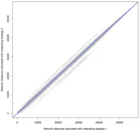
The following R commands (snippet 10) calculate the network distances between each pair of
London property locations with LN.ig1 and LN.ig2, reflecting the two different point integration
strategies used. The resultant matrices are different but highly correlated, as depicted in the
scatterplot of Figure 12. Observe that the corresponding vertices of the input locations are marked
with their orders returned by the function points2network, which provides an assessment of accuracy.
Figure 12. Network distances calculated with two different integrating strategies (London case study).
Code snippet 10:
# Strategy 1
LN.pt.VIDs1 <‐ as.numeric(LN.pt2nt1[[3]])
V.idx1 <‐ as.numeric(levels(as.factor(LN.pt.VIDs1)))
ND.mat1 <‐ shortest.paths(LN.ig1, v = LN.pt.VIDs1, to = V.idx1) ND.mat1 <‐ ND.mat1[, match(LN.pt.VIDs1, V.idx1)]
# Strategy 2
LN.pt.VIDs2 <‐ as.numeric(LN.pt2nt2[[3]])
V.idx2 <‐ as.numeric(levels(as.factor(LN.pt.VIDs2)))
ND.mat2 <‐ shortest.paths(LN.ig2, v = LN.pt.VIDs2, to = V.idx2) ND.mat2 <‐ ND.mat2[, match(LN.pt.VIDs2, V.idx2)]
# Scatterplot
plot(ND.mat1, ND.mat2, pch = 16, cex = 0.2, col = “grey”, xlab = “Network distances calculated with integrating strategy 1”, ylab = “Network distances calculated with integrating strategy 2”)
abline(a = 0, b = 1, col = “blue”, lwd = 2)
In addition, the corresponding travel time distances for the London case study can be calculated
with the converted graphs, LN.ig3 and LN.ig4, using the following R commands (snippet 11):
Figure 12.Network distances calculated with two different integrating strategies (London case study).
Code snippet 10:
# Strategy 1
LN.pt.VIDs1 <- as.numeric(LN.pt2nt1[[3]])
V.idx1 <- as.numeric(levels(as.factor(LN.pt.VIDs1)))
ND.mat1 <- shortest.paths(LN.ig1, v = LN.pt.VIDs1, to = V.idx1) ND.mat1 <- ND.mat1[, match(LN.pt.VIDs1, V.idx1)]
# Strategy 2
LN.pt.VIDs2 <- as.numeric(LN.pt2nt2[[3]])
V.idx2 <- as.numeric(levels(as.factor(LN.pt.VIDs2)))
ND.mat2 <- shortest.paths(LN.ig2, v = LN.pt.VIDs2, to = V.idx2) ND.mat2 <- ND.mat2[, match(LN.pt.VIDs2, V.idx2)]
# Scatterplot
plot(ND.mat1, ND.mat2, pch = 16, cex = 0.2, col = “grey”, xlab = “Network distances calculated with integrating strategy 1”, ylab = “Network distances calculated with integrating strategy 2”)
abline(a = 0, b = 1, col = “blue”, lwd = 2)
In addition, the corresponding travel time distances for the London case study can be calculated with the converted graphs,LN.ig3andLN.ig4, using the followingRcommands (snippet 11):
Code snippet 11:
# Strategy~1
TT.mat1 <- shortest.paths(LN.ig3, v = LN.pt.VIDs1, to = V.idx1) TT.mat1 <- ND.mat1[, match(LN.pt.VIDs1, V.idx1)]
# Strategy 2
TT.mat2 <- shortest.paths(LN.ig2, v = LN.pt.VIDs2, to = V.idx2) TT.mat2 <- TT.mat2[, match(LN.pt.VIDs2, V.idx2)]
ISPRS Int. J. Geo-Inf.2018,7, 293 16 of 19
ISPRS Int. J. Geo‐Inf. 2018, 7, x FOR PEER REVIEW 15 of 18
Code snippet 11:
# Strategy 1
TT.mat1 <‐ shortest.paths(LN.ig3, v = LN.pt.VIDs1, to = V.idx1) TT.mat1 <‐ ND.mat1[, match(LN.pt.VIDs1, V.idx1)]
# Strategy 2
TT.mat2 <‐ shortest.paths(LN.ig2, v = LN.pt.VIDs2, to = V.idx2) TT.mat2 <‐ TT.mat2[, match(LN.pt.VIDs2, V.idx2)]
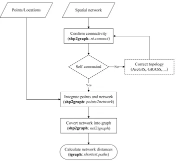
As a useful summary of this work, a flow chart for calculating network distances with shp2graph
and igraph is given in Figure 13.
Figure 13. Flow chart of calculating network distances with shp2graph and igraph.
3.5. Example Extensions
Shortest paths can also be found via the following set of R commends (snippet 12) for the Ontario
road data where the function shortest.paths is replaced with get.shortest.paths. Here, an interactive
experiment was conducted to find the shortest path between any pair of locations randomly inputted
and the result is given in Figure 14.
Code snippet 12:
plot(ORN.nt) coords <‐ locator(2)
coords <‐ cbind(coords$x, coords$y) points(coords, pch = 3, col = “red”)
pt2nt1 <‐ points2network(ntdata = ORN.nt, pointsxy = coords, Detailed = T, ELComputed = T, approach = 2, ea.prop = rep(0, 2))
V.idx3 <‐ as.numeric(pt2nt1[[3]])
Figure 13.Flow chart of calculating network distances withshp2graphandigraph.
3.5. Example Extensions
Shortest paths can also be found via the following set of R commends (snippet 12) for the Ontario road data where the functionshortest.pathsis replaced withget.shortest.paths. Here, an interactive experiment was conducted to find the shortest path between any pair of locations randomly inputted and the result is given in Figure14.
Code snippet 12:
plot(ORN.nt)
coords <- locator(2)
coords <- cbind(coords$x, coords$y) points(coords, pch = 3, col = “red”)
pt2nt1 <- points2network(ntdata = ORN.nt, pointsxy = coords, Detailed = T, ELComputed = T, approach = 2, ea.prop = rep(0, 2))
V.idx3 <- as.numeric(pt2nt1[[3]])
V.coords <- cbind(pt2nt1[[4]][V.idx3], pt2nt1[[5]][V.idx3]) points(V.coords, pch = 16, col = “green”)
lines(rbind(coords[1,], V.coords[1,]), lty = 2, col = “blue”) lines(rbind(coords[2,], V.coords[2,]), lty = 2, col = “blue”) igr3 <- nel2igraph(pt2nt1[[1]], pt2nt1[[2]], weight = pt2nt1[[8]])
path <- get.shortest.paths(igr3, from = V.idx3[1], to = V.idx3[2])$vpath[[1]] for(i in 1:(length(path)-1))
ISPRS Int. J. Geo-Inf.2018,7, 293 17 of 19
ISPRS Int. J. Geo‐Inf. 2018, 7, x FOR PEER REVIEW 16 of 18
V.coords <‐ cbind(pt2nt1[[4]][V.idx3], pt2nt1[[5]][V.idx3]) points(V.coords, pch = 16, col = “green”)
lines(rbind(coords[1,], V.coords[1,]), lty = 2, col = “blue”) lines(rbind(coords[2,], V.coords[2,]), lty = 2, col = “blue”) igr3 <‐ nel2igraph(pt2nt1[[1]], pt2nt1[[2]], weight = pt2nt1[[8]])
path <‐ get.shortest.paths(igr3, from = V.idx3[1], to = V.idx3[2])$vpath[[1]] for(i in 1:(length(path)‐1))
lines(cbind(pt2nt1[[4]][path[i,i+1]], pt2nt1[[5]][path[i,i+1]]), lwd =2, col = “blue”)
Figure 14. An interactive example for finding the shortest path with shp2graph and igraph (Ontario
road data).
Furthermore, the igraph package provides a vast collection of graph handling and analysis
tools—i.e., not just tools to calculate network distances and shortest paths, as demonstrated here. The
following R code (snippet 13) showcases some extensions for shp2graph via igraph, such as
calculating vertex and edge ‘betweeness’ and network diameter (as shown in Figure 15), or
measuring network connectivity [38].
Code snippet 13:
V.bn <‐ betweenness(igr2) E.bn <‐ edge_betweenness(igr2) G.dm <‐ diameter(igr2, directed = F) V.gdm <‐ get_diameter(igr2, directed = F) plot(ORN.nt)
for(i in 1:(length(V.gdm)‐1))
lines(cbind(rtNEL2[[6]][V.gdm [i,i+1]], rtNEL2[[7]][V.gdm[i,i+1]]), lwd = 2, col = “red”)
Figure 14.An interactive example for finding the shortest path withshp2graphandigraph(Ontario
road data).
Furthermore, theigraphpackage provides a vast collection of graph handling and analysis tools—i.e., not just tools to calculate network distances and shortest paths, as demonstrated here. The followingRcode (snippet 13) showcases some extensions forshp2graphviaigraph, such as calculating vertex and edge ‘betweeness’ and network diameter (as shown in Figure15), or measuring network connectivity [38].
ISPRS Int. J. Geo‐Inf. 2018, 7, x FOR PEER REVIEW 17 of 18
Figure 15. Finding the network diameter with shp2graph and igraph (Ontario road data).
4. Summary
In this study, the R package shp2graph is demonstrated. It provides a set of tools to convert a
spatial network into an ‘igraph’ graph of the igraph R package and in doing so, allows the rich set of
graph handling and analysis tools in igraph to be available for a spatial network analysis, all within
the R statistical computing environment. In particular, a route map for calculating road network
distances for three urban case studies is presented, where functions from both shp2graph and igraph
are described and applied. The calculation of travel time distances by weighting edges of the
converted graph with travel costs is also presented. The shp2graph package continues to evolve,
where tools such as those for topology correction and spatial indexing for improved computation
times are in current development.
Author Contributions: B.L. conceived and designed the study; M.C. helped develop shp2graph, performing
experiments and analyses; M.X. validated all the experiments and codes; H.S. made suggestions and provided
project administration for funding this study; B.L. wrote the manuscript assisted by P.H.
Funding: Natural Science Foundation of China grant number [NSFC: U1533102] and an open Research Fund
Program of Shenzhen Key Laboratory of Spatial Smart Sensing and Services (Shenzhen University)
Conflicts of Interest: The authors declare no conflict of interest.
References
1. Barthélemy, M. Spatial networks. Phys. Rep. 2011, 499, 1–101.
2. Lu, B.; Charlton, M. Convert a Spatial Network to a Graph in R. In Proceedings of the R User Conference,
Coventry, UK, 16–18 August 2011.
3. George, B.; Shekhar, S. Road maps, digital. In Encyclopedia of GIS; Shashi, S., Hui, X., Eds.; Springer: New
York, NY, USA, 2008.
4. Goodchild, M.F. Geographical data modeling. Comput. Geosci. 1992, 18, 401–408.
5. Gastner, M.T.; Newman, M.E.J. The spatial structure of networks. Eur. Phys. J. B Condens. Matter Complex Syst. 2006, 49, 247–252.
6. Fowler, P.A. The königsberg bridges—250 years later. Am. Math. Mon. 1988, 95, 42–43.
7. Appert, M.; Chapelon, L. The space‐time variability of road base accessibility: Application to london. In Graphs and Networks; Mathis, P., Ed.; ISTE: London, UK, 2007; pp. 3–28.
8. R Core Team. R: A Language and Environment for Statistical Computing; R Foundation for Statistical
Computing: Vienna, Austria, 2017.
Figure 15.Finding the network diameter withshp2graphandigraph(Ontario road data).
Code snippet 13:
ISPRS Int. J. Geo-Inf.2018,7, 293 18 of 19
V.gdm <- get_diameter(igr2, directed = F) plot(ORN.nt)
for(i in 1:(length(V.gdm)-1))
lines(cbind(rtNEL2[[6]][V.gdm [i,i+1]], rtNEL2[[7]][V.gdm[i,i+1]]), lwd = 2, col = “red”)
4. Summary
In this study, theRpackageshp2graphis demonstrated. It provides a set of tools to convert a spatial network into an ‘igraph’ graph of theigraph Rpackage and in doing so, allows the rich set of graph handling and analysis tools inigraphto be available for a spatial network analysis, all within theRstatistical computing environment. In particular, a route map for calculating road network distances for three urban case studies is presented, where functions from bothshp2graphandigraph are described and applied. The calculation of travel time distances by weighting edges of the converted graph with travel costs is also presented. Theshp2graphpackage continues to evolve, where tools such as those for topology correction and spatial indexing for improved computation times are in current development.
Author Contributions: B.L. conceived and designed the study; M.C. helped developshp2graph, performing
experiments and analyses; M.X. validated all the experiments and codes; H.S. made suggestions and provided project administration for funding this study; B.L. wrote the manuscript assisted by P.H.
Funding:Natural Science Foundation of China grant number [NSFC: U1533102] and an open Research Fund
Program of Shenzhen Key Laboratory of Spatial Smart Sensing and Services (Shenzhen University).
Conflicts of Interest:The authors declare no conflict of interest.
References
1. Barthélemy, M. Spatial networks.Phys. Rep.2011,499, 1–101. [CrossRef]
2. Lu, B.; Charlton, M. Convert a Spatial Network to a Graph in R. In Proceedings of the R User Conference, Coventry, UK, 16–18 August 2011.
3. George, B.; Shekhar, S. Road maps, digital. InEncyclopedia of GIS; Shashi, S., Hui, X., Eds.; Springer: New York, NY, USA, 2008.
4. Goodchild, M.F. Geographical data modeling.Comput. Geosci.1992,18, 401–408. [CrossRef]
5. Gastner, M.T.; Newman, M.E.J. The spatial structure of networks.Eur. Phys. J. B Condens. Matter Complex Syst.
2006,49, 247–252. [CrossRef]
6. Fowler, P.A. The königsberg bridges—250 years later.Am. Math. Mon.1988,95, 42–43.
7. Appert, M.; Chapelon, L. The space-time variability of road base accessibility: Application to london. InGraphs and Networks; Mathis, P., Ed.; ISTE: London, UK, 2007; pp. 3–28.
8. R Core Team.R: A Language and Environment for Statistical Computing; R Foundation for Statistical Computing: Vienna, Austria, 2017.
9. Lu, B.; Charlton, M.; Harris, P.; Fotheringham, A.S. Geographically weighted regression with a non-euclidean distance metric: A case study using hedonic house price data. Int. J. Geogr. Inf. Sci. 2014,28, 660–681. [CrossRef]
10. Van Etten, J. R package gdistance: Distances and routes on geographical grids.J. Stat. Softw.2017,1. [CrossRef] 11. Pebesma, E.J.; Bivand, R.S. Classes and methods for spatial data in R.R News2005,5, 9–13.
12. ESRI Corp.Arcgis Desktop: Release 10; Environmental Systems Research Institute: Redlands, CA, USA, 2011. 13. GRASS Development Team.Geographic Resources Analysis Support System (Grass GIS) Software; Open Source
Geospatial Foundation: Chicago, IL, USA, 2018.
14. pgRouting Community. Pgrouting 2.3. Available online:https://pgrouting.org/index.html(accessed on 5 May 2018).
15. Boeing, G. Osmnx: New methods for acquiring, constructing, analyzing, and visualizing complex street networks.Comput. Environ. Urban Syst.2017,65, 126–139. [CrossRef]
ISPRS Int. J. Geo-Inf.2018,7, 293 19 of 19
17. Hagberg, A.; Swart, P.; S Chult, D. Exploring Network Structure, Dynamics, and Function Using NetworkX. In Proceedings of the 7th Python in Science Conference, Pasadena, CA, USA, 19–24 August 2008.
18. Karduni, A.; Kermanshah, A.; Derrible, S. A protocol to convert spatial polyline data to network formats and applications to world urban road networks.Sci. Data2016,3, 160046. [CrossRef] [PubMed]
19. Furieri, A.Spatialite-Tools, 2017-03-03 ed.; SpatiaLite: Genova, Italy, 2018.
20. Jiang, B.Axwoman 6.3: An Arcgis Extension for Urban Morphological Analysis; University of Gävle: Gävle, Sweden, 2015.
21. Gollini, I.; Lu, B.; Charlton, M.; Brunsdon, C.; Harris, P. Gwmodel: An R package for exploring spatial heterogeneity using geographically weighted models.J. Stat. Softw.2015,63, 1–50. [CrossRef]
22. Lu, B.; Harris, P.; Charlton, M.; Brunsdon, C. The gwmodel r package: Further topics for exploring spatial heterogeneity using geographically weighted models.Geo-Spat. Inf. Sci.2014,17, 85–101. [CrossRef] 23. Csardi, G.; Nepusz, T. The igraph software package for complex network research.InterJournal Complex Syst.
2006,1695, 1–9.
24. Dijkstra, E.W. A note on two problems in connexion with graphs.Numer. Math.1959,1, 269–271. [CrossRef] 25. Bellman, R. On a routing problem.Q. Appl. Math.1958,16, 87–90. [CrossRef]
26. Ford, L.R.Network Flow Theory; RAND Corporation: Santa Monica, CA, USA, 1956.
27. Johnson, D.B. Efficient algorithms for shortest paths in sparse networks.J. ACM1977,24, 1–13. [CrossRef] 28. Mathis, P. (Ed.) Strengths and deficiencies of graphs for network description and modeling. InGraphs and
Networks; ISTE: London, UK, 2007; p. xvi.
29. Peterborough, O.Ontario Road Network; Ontario Ministry of Natural Resources: Peterborough, ON, Canada, 2006. 30. Mainguenaud, M. Modelling the network component of geographical information systems.Int. J. Geogr.
Inf. Syst.1995,9, 575–593. [CrossRef]
31. Jiang, B.; Claramunt, C. A structural approach to the model generalization of an urban street network. Geoinformatica2004,8, 157–171. [CrossRef]
32. Viana, M.P.; Strano, E.; Bordin, P.; Barthelemy, M. The simplicity of planar networks.Sci. Rep.2013,3, 3495. [CrossRef] [PubMed]
33. Boeing, G. Planarity and street network representation in urban form analysis.arXiv2018, arXiv:1806.01805. [CrossRef]
34. Abdulganiev, I.; Agafonov, A. Automatic Checking of Road Network Models. In Proceedings of the CEUR Workshop Proceedings, Moscow, Russia, 25–26 November 2016; pp. 249–255.
35. OpenStreetMap.Estevan Road Network; OpenStreetMap Community: London, UK, 2014.
36. Wade, T.; Sommer, S.A to Z GIS: An Illustrated Dictionary of Geographic Information Systems; ESRI Press: Redlands, CA, USA, 2006.
37. Tchoukanski, I.Et Geotools; 11.5; ET SpatialTechniques: Faerie Glen, South Africa, 2018.
38. Knight, P.L.; Marshall, W.E. The metrics of street network connectivity: Their inconsistencies.J. Urban. Int. Res. Placemarking Urban Sustain.2015,8, 241–259. [CrossRef]