JEA, An Interactive Optimisation Engine for Building Energy Performance Simulation
Yi Zhang
1, Lubo Jankovic
21
Energy Simulation Solutions Ltd, Leicester, United Kingdom
2Birmingham School of Architecture and Design, Birmingham City University, Birmingham,
United Kingdom
Abstract
This paper presents the motivation, concept and implementation of a new interactive optimisation engine designed to be generic and be able to work with different building simulation tools. The key technological advances are the full interactivity and collaboration features built around a multi-objective optimisation algorithm that is fine-tuned for building design applications. The interactive features, including the ability to change optimisation criteria, search space and evaluation models on-the-fly, are unheard-of in other optimisation tools. An example design task is used to demonstrate the capability and advantages of these unique features.
Introduction
Optimisation has gained increasing attention amongst researchers and practitioners in the built environment. Many applications of optimisation techniques and development of tools incorporating optimisation functions have been reported in the area of building design. However, optimisation tools that are efficient for a broad range of applications, yet simple enough to use without the requirement of prior knowledge of optimisation, are hard to find.
Another critical issue with the current optimisation tools is that to most users, they work as a black box. Once set up and running, the user cannot do much else except waiting to see if they get the desired results in the end or not. Innocent errors in the problem's setup or in the configuration of the algorithms can easily lead to significant time losses.
In order to address these limitations, a brand new optimisation engine named JEA has been developed for building simulation users. The engine is operated by a set of standard APIs that are agnostic about simulation models or tools. It offers interactive control over algorithm configurations and optimisation problem definitions. Changes can be made on-the-fly without stopping the optimisation process. The engine can also be accessed via internet protocols to facilitate online and collaborative optimisation projects. These features are only possible because of key advances in the development of the algorithms and the problem representations, which will be described in the article. An example building design project is presented to demonstrate the advantages of using the new optimisation engine.
An interactive approach
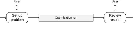
As a decision-making process, design is intrinsically interactive and iterative. In order to use optimisation as an integral tool in the design processes, the users must have sufficient level of control over how the optimisation process works. Figure 1 shows the typical way that the optimisation process is used. In the three steps, the user has control over the setting up of the optimisation problem, and the analysis of the results, but has very limited opportunity to intervene during the optimisation run.
Figure 1: Traditional optimisation process For building design applications, the optimisation run can take significant amount time depending on the complexity of the models and the design task. Quite often the process has to be restarted due to errors (or changes) in the problem setup, which inevitably leads to time loss.
A solution to this issue is to allow the design problem set up to be reviewed and revised during the optimisation process, as illustrated in Figure 2. In this way, errors can be corrected, and changes of design context can be incorporated without abandoning the current progress.
Figure 2: Interactive optimisation process Substantial changes must be made to the optimisation algorithms and the representation of the problems to achieve such interactivity. The following sections of the paper describe how it works and how it can be used to achieve the most flexible and efficient workflow.
The optimisation engine
GenOpt (Wetter, 2001) and MOBO (Palonen et al. 2013) are two established generic optimisation tools, each incorporating a range of algorithms and the ability to work with a number of building simulation programs. Our development, the JEA engine, differs from them in
Optimisation run
Set up problem
Review results
User User
Optimisation run
Set up problem
Review results
User User
Adjust goals and search space
two ways. First, the JEA engine provides only the search algorithms, and the associated data representation for the optimisation problems. It does not include model manipulation or result extraction functions to work with simulation tools such as EnergyPlus. Instead, developers can use the engine to develop their own tools for specific optimisation applications.
Second, the JEA engine offers only one optimisation algorithm instead of multiple choices. It is a constrained multi-objective algorithm based on Evolutionary Algorithms (EAs) and has been tuned for a broad range of problems found in applications in the built environment. This removes the confusion of which algorithm to choose for users. On the other hand, additional methods such as parametric analysis and uncertainty/sensitivity analysis are provided to aid the interactive design approach.
Briefly, the new engine has features include:
highly efficient and versatile multi-objective optimisation algorithm based on the EAs, with flexible constraint handling strategy
suitable for both multi-objective and single objective problems, constrained or unconstrained
enabling full interactivity with on-the-fly adjustment of algorithm configuration, search space, optimisation criteria, and the evaluation models
simple JSON based Application Programing Interface (API) providing complete control of the engine, and data access for progress monitoring, solution inspection, and algorithm analysis.
Optimisation Process
Evolutionary Algorithms (EAs) are a well-known group of nature inspired algorithms for operational research. The methods, their strengths and limitations, are extensively covered in the literature, such as (Bäck, 1996). EA was chosen as the main algorithm in JEA, for its robustness, versatility and efficiency in handling mixed continuous and discrete, constrained, nonlinear, multimodal, multi-objective problems often seen in building applications.
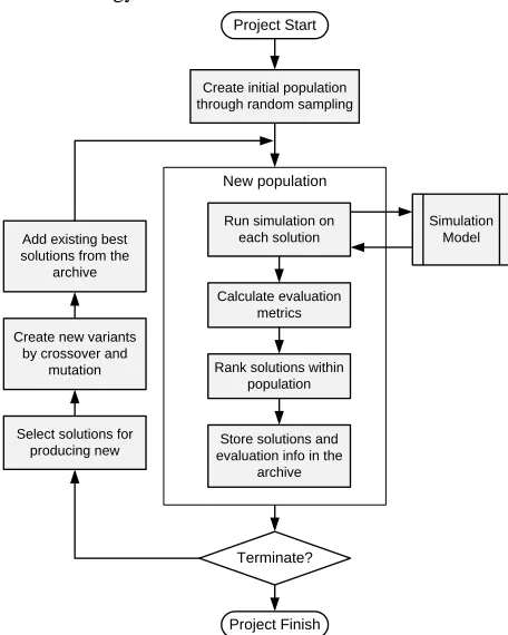
Figure 3 shows an overview of the EA process implemented in JEA. Each EA process (project) starts with initializing the engine instance and creating the first set of solutions based on random sampling. The solutions are evaluated, using external simulation models if necessary, and ranked based on the optimisation criteria. "Good" solutions are selected for generating new cases using the crossover and mutation operators, and continue going through the evolution cycle until one of the termination criteria is met.
The EA process is "generation" based, i.e. there is a clear starting point for each iteration. This gives the opportunity for applying user interaction, which we will discuss in length in this paper. Before that, let us first look at the three techniques that are essential for achieving the efficacy and interactivity in JEA: the integer-based encoding scheme, the constrained
multi-objective ranking method, and the Pareto archived global elitism strategy.
Figure 3: The EA process as implemented in JEA
Integer-based Encoding Scheme
Three encoding schemes are commonly used in the EAs: binary encoding, integer encoding, and real value encoding. Real value encoding not only represents a solution using the problem variables’ native values, continuous or discrete, it can also capture the relationship between variables by imposing a data structure (such as a tree in the case of Genetic Programming). To take advantage of real value encoding, prior knowledge of the problem is essential, and the problem-specific operators should be used, which makes it less suitable for generic optimisation engines.
The optimisation problems in building design normally have both discrete (e.g. window construction types) and continuous variables (e.g. insulation thickness), albeit the continuous variables rarely require high resolutions. Considering the depth of shading overhang, for example, a value of 1.123m does not differ much from either 1.10m or 1.15m in the practical sense, due to the presence of measurement and other uncertainties.
Binary encoding is canonical to Genetic Algorithms. A solution is represented by a string of binary digits (bits). If 10 bits are used to encode one continuous variable, it is effectively discretized into 1024 values with the variable's given domain. The benefit of using binary encoding is that the algorithm can use a standard set of crossover and mutation operators, disregarding the problem it is solving. The drawbacks, however, are that
Create initial population through random sampling
Project Start
New population
Run simulation on each solution
Calculate evaluation metrics
Rank solutions within population
Store solutions and evaluation info in the
archive Create new variants
by crossover and mutation
Select solutions for producing new Add existing best solutions from the
archive
Terminate?
Simulation Model
the mapping between the encoding and the actual values is not intuitive and often inefficient.
Integer encoding represents a solution with the indices of the values of each design variables. This representation is natural for discrete variables, whose values are already defined as a list. For continuous variables, however, the user needs to specify the values to use manually. For example, the values for the depth of overhang must be defined as 0.0, 0.1, 0.2, up to 1.0, instead of to just give the range [0.0, 1.0]. The reward of making the extra effort is that the algorithm will not waste time on chasing the minute increments between the specified values, leading to much faster convergence (Zhang, 2012). In JEA, the integer encoding is the method of choice.
Constrained Multi-objective Ranking
The ranking method determines how the EA judges the relative quality of the solutions. JEA uses Non-dominated Sorting from NSGA-II (Deb et al. 2002), integrated with Stochastic Ranking (Runarsson and Yao, 2000), for constrained multi-objective problems.
NSGA-II is one the best known and widely used algorithms for multi-objective optimisation. The key trick is the Non-dominated Sorting method (hence the name), which is proven to be highly effective in ranking competing objectives. It also works well with single-objective problems, which makes it perfect for our purpose. One deficiency of the original NSGA-II algorithm, however, is that it does not provide a way of efficient constraint handling.
Constraint handling is a topic that attracts lots of attention from algorithm designers. The efficiency of constraint handling is measured by not only how quickly feasible solutions are found, but also the quality of those feasible solutions. If a strategy pushes too hard for meeting the constraints, it may hamper exploration for better objective values. On the other hand, if it is too lenient, too much time may be wasted on infeasible solutions. The balance depends on the nature of the problem, so a perfect strategy may not exist. However, from our research we found one of the best strategies in terms of robustness of adaptability to different problems, is Stochastic Ranking.
Stochastic Ranking is a probabilistic strategy to rank solutions according to different objective and constraint functions. Its original form is designed for one objective against one constraint. In order to make it work with NSGA-II, the following steps are taken:
1. All constraints are scaled (normalised) and then aggregated so that the infeasibility (constraint violations) is measured as a value in [0, 1].
2. Infeasibility is used as an additional objective and sorted with Nondominated Sorting with all other objectives. This produces an initial ranking order of all solutions.
3. Stochastic Ranking is then applied to the initial rank of each solution (treated as its objective value) and
its aggregated infeasibility value. This produces the final ranking of the solutions.
The benefit of this slightly complex arrangement is that it works well with problems with any number of objectives (including single objective) and constraints, and unconstrained problems. The user can use a single parameter, what we call "Objective Bias", to control the level of the push for feasibility.
Pareto Archived Global Elitism
Evolutionary algorithms are stochastic in nature. The user has little control over which direction or what solutions to explore next. Quite often promising solutions may appear in one generation and then disappear for good in the subsequent iterations. Elitism is a method for preserving good solutions. Basically, it selects cases from a pool of known solutions and inserts them back into the working population.
In Pareto Archived Elitism, all known solutions on the global Pareto Front are stored. They form the pool from which the elitism operator picks "elites". In JEA, the maximum number of elites and whether they can include infeasible solutions can be controlled by parameters. The combination of the encoding scheme, the ranking method, and the elitism strategy makes JEA highly effective in solving complex optimisation problems, which we have seen in many examples. Since we are developing a separate paper to compare JEA with other optimisation algorithms, it will not be discussed here for the time being.
Implementation of Interactivity
The main advances we have achieved with JEA is the interactivity, i.e. the ability user has to adjust or modify the optimisation process when it is running. To the authors' knowledge, no other optimisation tools have achieved the same level of on-the-fly interactivity as JEA has.
We consider that there is five levels of interactivity, ordered by increasing complexity to implement: (1) progression control, (2) algorithm settings, (3) evaluation metrics, (4) search space, and (5) evaluation model. Most existing optimisation tools has partial progression control (level 1). For example, in GenOpt the user can start and stop an optimisation process at will. Many EA-based tools, MOBO included, has live algorithm settings control (level 2), which means the user can change algorithm settings on-the-fly. In this part of the paper, we explain in detail what the different interactivity levels are and how they are implemented.
Level 1: Progression Control
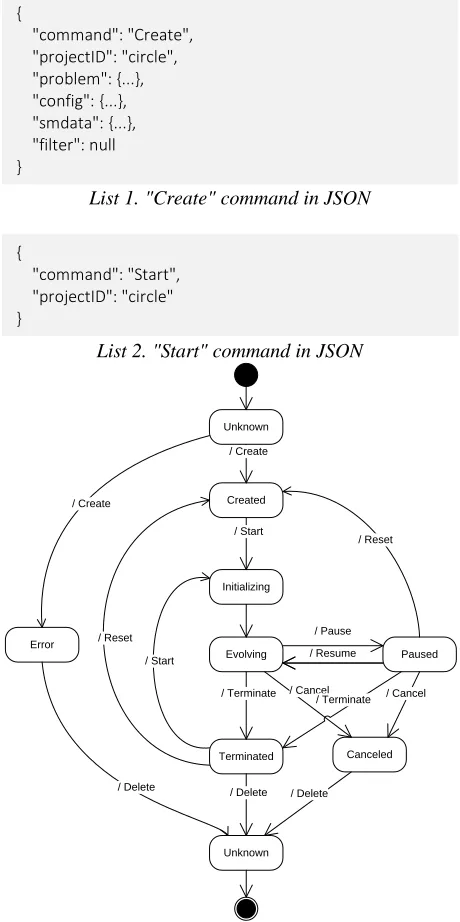
system at the end of each iteration. The stored states can then be used to resume the process on user's request. The EA process (referred to as the "project") can be controlled using a set of commands following the form as in List 1, which contains the command, a project ID, and further data fields. The "problem", "config", "smdata" and "filter" fields are optional and can be omitted. In fact, only the "Create", "Update" and "Report" commands need the additional fields. List 2 shows an example "Start" command.
List 1. "Create" command in JSON
List 2. "Start" command in JSON
Figure 4: State flow of an EA project and commands The full set of commands for JEA include "Create", "Update", "Start", "Pause", "Resume", "Terminate", "Cancel", "Reset", and "Delete" for procession control, plus "Status", "Report", and "Data" for data access. Figure 4 shows the state flow of the EA project and the corresponding commands.
Level 2: Algorithm Settings
EAs are highly customizable heuristic algorithms. This is considered a significant advantage by experienced users, as they can tailor the algorithm to suit the characters of the problem at hand. However, very few users can tell immediately what configuration of the algorithm would work best for a new project. The ability to adjust settings after seeing how the algorithm behaves is very useful to users.
The current version of JEA supports on-the-fly update of the following parameters:
Search method: optimisation (NSGA-II), exhaustive search (Parametrics), or random sampling
Population sizes: adjustable depending on the complexity of the problem and the available computing resources/budget.
Reproduction: crossover and mutation rates
Selection pressure: tournament size
Constraint handling: ranking bias between constraints and objectives
Elitism strategy: tolerance for infeasible solutions
Termination criteria: number of iterations, time and cost budget.
It is worth noting that the ability to switch between different algorithms, e.g. from NSGA-II to full parametrics and back, is probably unique to JEA. The reasons for doing this is explained in the use case. List 3 is an example algorithm configuration.
List 3. Algorithm configuration example
Level 3: Evaluation Metrics
In each iteration of the optimisation process, assessing and comparing the quality of the competing solutions is done by calculating the evaluation metrics (objective and constraint functions) from the simulation results. The evaluation metrics are then used by the the optimisation algorithm to rank existing solutions for producing new solutions. Sophisticated ranking methods are often necessary for dealing with multi-criteria optimisation problems.
In an optimisation project, the actual design goals are expressed in the form of objective and constraint Unknown
Unknown Initializing Created
Evolving Paused
/ Pause
Terminated Canceled
/ Delete / Delete Error
/ Terminate / Cancel / Cancel / Create
/ Start
/ Resume / Start
/ Reset
/ Terminate / Create
/ Delete
/ Reset
"config": {
"algorithm": "NSGA2", "sampleSize": 0,
"sampleOption": "RANDOM", "initPopSize": 10,
"evolvePopSize": 10, "maxPopSize": 10000, "mutationRate": 0.2, "crossoverRate": 1, "tournamentSize": 2, "objectiveBias": 0, "elitismTolerance": 0, "maxGenerations": 100, "maxEvaluations": 1000, "maxComputingTime": 100, "maxWallTime": 24 }
{
"command": "Start", "projectID": "circle" }
{
functions. For example, if energy performance, comfort level and cost are of concern, three objectives may be assigned to the optimisation problem, i.e. "to minimise energy consumption, discomfort and cost". However, any of the following formulations are possible, too:
to minimise energy consumption and discomfort, subject to limited cost (two objectives and one constraint);
to minimise cost, subject to energy consumption and discomfort not exceeding certain levels, respectively (one objective, two constraints); or even,
to find any solution that energy consumption, discomfort and cost are all below their respective limit (no objective, three constraints).
There are apparently more ways to formulate the problem, and they can be equivalent from the user's point of view. However, optimisation algorithms may treat constraints and objectives in very different ways, depending on the ranking methods used. The formulation of the optimisation problem affects how the search process progresses, therefore has a significant impact on the solutions, and how quickly they are found. Choosing the right objectives and constraints for a project is not easy for even the most experienced users. Furthermore, the design criteria may change due to the emergence of new information or on client's request. The ability to adjust the evaluation metrics on-the-fly helps the user to avoid losing all solutions that have been explored when such changes happen. JEA will simply adopt the new metrics and re-rank the existing solutions without interrupting the optimisation process.
There are three types of evaluation metrics the user can specify in JEA:
User Metrics ("userMetrics") are values calculated from simulation results for user's own reference only. They can be visualised, but not used in the optimisation process.
Objectives ("objectives") are values to be minimised or maximised by the optimisation process.
Constraints ("constraints") are values with a defined acceptable range. The optimisation process will try to push solutions to fall within this range.
List 4 shows an example of evaluation metrics definition. The only constraint ("s1") in the example calculates the geometrical distance of the solution to the point (50, 50), and requires the distance to be less than 30. If the distance is larger than 30, a penalty is applied to the solution. Since computing of the evaluation metrics is trivial, they can be recalculated whenever necessary. The user can submit new metric definitions by calling the "Update" command.
List 4. Evaluation metrics definition example
Level 4: Search Space
Another common challenge in setting up optimisation problem is deciding on the search space. The search space for optimisation is defined by the available options of each design variables. Normally the larger (more options) the search space is, the longer it takes to find the optimal solutions. Performing a global sensitivity analysis may help to eliminate less important variables. The likely regions where optimal solutions are may also emerge from experimenting with the model. The latter is more akin to the human design process.
For optimisation, level 4 interactivity means that the search space of the optimisation problem can be adjusted during the process. The user can change the definition of the design variables, e.g. by adding or removing options in the variables, or even adding or removing variables in the optimisation problem. The challenge for the algorithm is to maintain encoding consistency of the existing solutions while incorporating variable definition changes.
JEA implements support for alternating search space by allowing the user to specify a "mask" to the initial search space. The mask defines a sub-space within the original search space. The algorithm operates within the effective
"userMetrics": [ { "name": "v1",
"caption": "User metric 1", "unit": "-",
"formula": "f1 + f2" }
],
"objectives": [ { "name": "t1",
"caption": "Objective 1", "unit": "-",
"direction": "Minimize", "formula": "f1" }, {
"name": "t2",
"caption": "Objective 2", "unit": "-",
"direction": "Minimize", "formula": "f2" }
],
"constraints": [ { "name": "s1",
"caption": "Constraint 1", "unit": "-",
"formula":
"Math.sqrt(Math.pow(f1-50, 2) + Math.pow(f2-50, 2))", "lb": 0,
"ub": 30, "min": 0, "max": 100, "weight": 1 }
search space, whereas all solutions are encoded in the original space to ensure encoding consistency.
Figure 5 shows the operations of refining the search space. It starts with the whole domain with a coarse mesh, progressing to smaller regions with finer meshes in three steps.
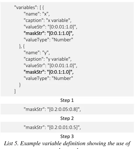
Figure 5: Result of exploring with different mesh sizes List 5 shows how this is done using the mask strings. In Step 1 the "valueStr" specifies the original search space, whereas the "maskStr" defines the same domain with a coarser mesh (0.1 vs. 0.01). In step 2 the mesh size is reduced to 0.05, at the same time the search boundary is reduced to [0.2, 0.8]. In step 3, Boundary and mesh size are further reduced to [0.2, 0.5] and 0.01, respectively.
Step 1
Step 2
Step 3
List 5. Example variable definition showing the use of value masks
The interactive control of the search space can have many uses, including layered and collaborated search strategies. These will be topics for future development.
Level 5: Evaluation Model
The ultimate level of interactivity is the ability to modify or change the model used for evaluating solutions. At present, it is not feasible to devise a consistent strategy for the optimisation algorithm to handle model changes.
Instead, the decision of what to do when a model is changed is delegated to the user.
JEA is implemented as a generic optimisation engine that is agnostic about which model or simulation tool is connected to it. To evaluate a solution, JEA sends a set of values for the corresponding design variables to the model, and expects a set of result values (see List 6 and 7) as defined in the optimisation project. How the result values have come about is not the engine's concern. If the model is changed by the user during the optimisation process, the user should decide whether the modification invalidate the existing solutions or not. If the impact is small, i.e. the ranking of the existing solutions would not differ much should all solutions be re-simulated, the optimisation process may carry on as before; otherwise, it may be better to start a new optimisation run.
List 6. Definition of evaluation results
Simulation request
Simulation result
List 7. Example data exchange between optimisation engine and simulation model
Why is model definition change useful, though? Having a model-unaware engine gives tool developers excellent opportunity to create hybrid optimisation approaches, which is essential for complex projects that require collaboration between multiple disciplines.
{
"name": "Gen-101", "projectName": "circle", "resultSet": {
"C-37_50": { "f1": 37, "f2": 50 }, "C-44_31": { "f1": 44, "f2": 31 }, ...
"C-41_22": { "f1": 41, "f2": 22 } }
} {
"name": "Gen-101", "projectName": "circle", "jobSet": {
"C-37_50": {"y": "0.5", "x": "0.37"}, "C-44_31": {"y": "0.31", "x": "0.44"}, ...
"C-41_22": {"y": "0.22", "x": "0.41"} },
"eventType": "Request" }
"evalResults": [ { "name": "f1",
"caption": "Model output 1", "unit": "-"
}, {
"name": "f2",
"caption": "Model output 2", "unit": "-"
} ]
"maskStr": "[0.2:0.01:0.5]", "maskStr": "[0.2:0.05:0.8]", "variables": [ {
"name": "x",
"caption": "x variable", "valueStr": "[0:0.01:1.0]", "maskStr": "[0:0.1:1.0]", "valueType": "Number" }, {
"name": "y",
"caption": "y variable", "valueStr": "[0:0.01:1.0]", "maskStr": "[0:0.1:1.0]", "valueType": "Number" }
Within one optimisation project, different models can be used to evaluate the solutions in many different ways. For example, EnergyPlus, TRNSYS, Radiance and Spreadsheets can be employed at the same time to assess different evaluation metrics of the same solution. Dynamic simulation models and simplified surrogates can be used alternatively to accelerate exploration. The output from one optimisation project can be the evaluation input of another, forming a hybrid algorithm. Even subjective assessment (e.g. on aesthetics) may be included in the optimisation process.
The implementation of model level interactivity, including the functions of running simulations and collecting results, needs to be done on the client's side by tool developers. And, more research is required to realise the full potential of the generic optimisation engine. Nevertheless, the new development has brought about possibilities that have never been seen before.
Optimisation as a Service
JEA may be accessed as a library, or online through its RESTful API. The online version that we call "Optimisation as a Service", or OAAS, further supports project sharing and collaboration.
With an online service on which the whole data set of an optimisation project is accessible from anywhere with internet connection, collaborations between a team of users would become possible. One useful scenario can be that an energy modeller creates the simulation model and sets up an optimisation project; the designer (architect, for example) operates the project to explore different design options, adjusting design criteria as needed, and instructs the modeller to make changes to the model when necessary. Advisors can be called in anytime when support is required, or the progress (in the form of a set of design solutions identified thus far) can be shown live to the clients.
Figure 6: Online optimisation service
The online optimisation service is accessed using HTTP requests to the service's URL. All operations described previously such as creating, updating, starting, pausing or cancelling an optimisation project are addressable following a REST pattern. For example, to start the project "MyProject", the request is:
List 8. Example RESTful API command for starting a project
For creating and updating operations, project definition and engine configuration data need to be sent to the server. In these cases, the requests must be must include the required data in JSON format as the payload. Examples of the requests are available online.
Once the optimisation process has started (with "Start" command), the engine will generate a set of cases awaiting simulation. The user, with a client software, instructs the server to retrieve the pending cases, run the simulations, and submit the results back to the server. On the server, the optimisation process will continue once all the expected results are received. In this arrangement, the user (with client software) is responsible for executing simulation and provide to the server with the expected results. The user can run simulations locally or use suitable online services, or input results manually. The main driver for the development of optimisation as an online service is to facilitate collaboration. Subject to the implementation in the client tools, it is possible for different users to collaborate by producing partial simulation results that collectively form the evaluation of the solutions. The access information of the service, the full details of the API and the example code are available at www.ensims.com/jea.
Example Application
We use a low energy building design case to demonstrate the key functions and the interactive process of the new optimisation engine. The case represents a challenging design task with multiple design goals, which are used interchangeably as constraints or as objectives to find the desirable solutions. The search space is gradually refined to accelerate the process. This example also gives a comparison between the new interactive approach and the traditional search strategies.
The Optimisation Problem
The model we used was developed as part of an on-going project on retrofitting residential houses to the Passivhaus standard. The houses to be retrofitted are of the type known as Wimpey No-Fines, characterised by concrete construction without the sand fraction. In the UK, approximately 300,000 dwellings were built using this method since the Second World War (Reeves and Martin, 1989). The original buildings had no thermal insulation.
Figure 7 shows the appearance of the actual houses and the model in DesignBuilder. The model was built using data from detailed site survey and then calibrated with utility bills (Jankovic and Basurra, 2016). Only one semi-detached house of the two is used in this example. online
j
EA
EA RESTful API
Project Data Store Model files
JSON
Designer
Modeller
Advisor / Observer
Figure 7: Houses to be retrofitted (from Jankovic and Basurra, 2016)
The task is to identify a set of retrofitting solutions encompassing a range of technical and behavioural parameters. From the decision maker's (e.g. the house owner's) point of view, there are three goals: reduce carbon emissions, improve comfort, and not to break the bank. The technical and behavioural parameters considered are listed in Table 1. The construction costs of all technical options are considered, despite that for the purpose of demonstration costs figures may not accurately reflect the present market price.
Table 1: Design Variables
Variable values count
Infiltration (ACH) 0.6, 1.0, 2.0, 3.0 4 Insulation (mm) 0, 100, 150... 270 6 Boiler (-) Gas, Biomass 2 Light fittings
(W/m2)
5.0, 3.0, 2.0, 1.0 4
PV east roof (%) 0% - 80% 9 PV west roof (%) 0% - 90% 10 Room Temp. (°C) 16.0, 16.5, ...,
24.0
17
Clothing (clo) 0.8, 0.9, ..., 1.4 7
Total: 2.06×10⁶
The total search space size of this project is just over 2 million, which is not a big problem for optimisation but well beyond the scope that a user can effectively explore manually. We want first to see if the optimisation algorithm in JEA is working correctly.
Efficacy of the Optimisation Algorithm
To test the effectiveness of the optimisation algorithm, we first run a random sample of 1,000 cases, whose carbon and cost metrics are shown in Figure 8a. We then
run JEA using the NSGA-II option with a population size of 10. Operational carbon emission and cost are used as two objectives, whereas discomfort hours (≤ 1,500hrs), according to ASHRAE55 Fanger's PMV model with designated clothing, is used as a constraint. After 500 cases have been evaluated, the result chart is shown in Figure 8b. The difference between Figure 8a and 8b is very clear.
a. 1,000 random sample
b. 500 optimisation output
Figure 8: Comparison between random sample and optimisation outputs
Looking at the best solutions found in both processes, at 100 evaluations, NSGA-II has already produced a set of results (circles in Figure 9) that are better than those from the 1,000 randomly selected cases (crosses in Figure 9), except the point at £20,000 and -0.2 tonne/year. Allowing the optimisation process to run to 500 evaluations, a set of 69 solutions emerges to form a clean off line between carbon and cost. This trade-off line (the "Pareto front") shows what has to be compromised in one objective, in order to meet the target in another. By inspecting the individual solutions, the user can gain insight on how design parameters impact on the objectives and constraints, too.
cost £17.8K, the reduction of £2.8K (14%) is significant.
Figure 9: Best solutions found in 500 and 100 evaluations using NSGA-II, and in 1,000 random sample Another indicator of the efficacy of NSGA-II is that in the random sample, only 277 of the 1,000 cases (28%) meet the comfort criterion, whereas, in the results of NSGA-II, 448 of the 500 cases (90%) evaluated to meet the same criterion. This shows that the optimisation algorithm in JEA handles constrained problems effectively.
Example of Search Manoeuvre
Next, we use an experiment to simulate a more complex use case on which the interactive features can be demonstrated. At the start the project, the same design criteria as in the previous section are used, i.e. carbon and cost as objectives, and discomfort hours as a constraint. In the middle of the project, the "client" changes their mind and no longer wants to install a biomass boiler. The new question is thus to find out whether carbon neutrality is achievable with the existing gas boiler, and what the minimum cost of the rest of retrofitting is. Some compromise on thermal comfort is acceptable.
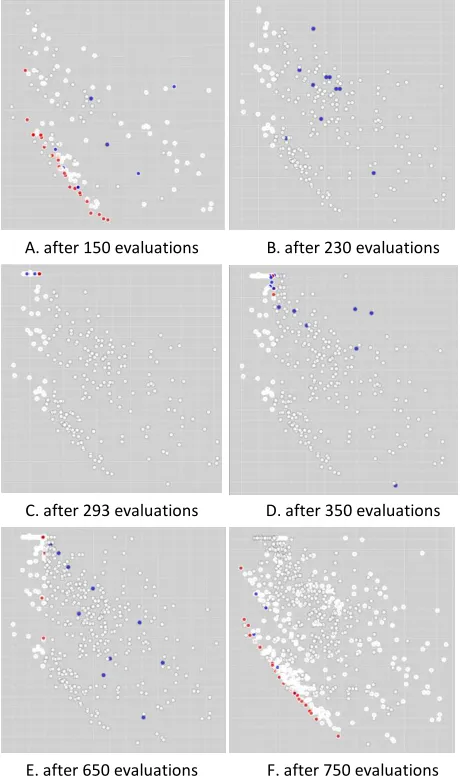
Here is how we did the experiment. The optimisation project starts as before. We assume that after 150 evaluations (Figure 10a), client's new instructions come in. The search space is adjusted by removing the biomass boiler option. We set cost and comfort as objectives, and carbon ≤ 0 as a constraint, to reflect the new requirement. After further 80 evaluations (Figure 10b), it becomes clear that "zero carbon" is a stringent constraint (this can be seen from the random sample), especially when one of the key low carbon technologies, biomass, is taken out. The optimisation engine may use a little help to find some feasible solutions first.
Using the pattern that has already emerged from the existing evaluations, and conventional wisdom, it is quite clear that throwing in all low-carbon technology and reducing heating demand to the minimum will give us the best chance to meet the zero carbon target. So we
pause the search process, apply masks to the design variables so that only the best air tightness, insulation, lighting, and maximum amount of PV are selected. Only the behavioural variables remain. We further limit the range of heating temperature setting to 16-20°C. The remaining size of the search space after masking is 63, small enough for an exhaustive search (a full parametric run). This method is the same principle as the "seeding" strategy in optimisation, where certain suboptimal solutions are inserted into the existing pool to influence the search process.
A. after 150 evaluations B. after 230 evaluations
C. after 293 evaluations D. after 350 evaluations
E. after 650 evaluations F. after 750 evaluations
Figure 10: Progress of the interactive experiment After "seeding" (Figure 10c), we have answered the first question: yes, the zero carbon target is achievable without a new biomass boiler. The next question is what the minimum cost is. The search space is reset to its original size except for biomass, and the search continues. Soon new (better) solutions emerge from the seeds (Figure 10d).
However, after another 300 evaluations (Figure 10e), the lowest cost solution found still costs nearly £24K, £4.5K (23%) higher than otherwise achievable with a new biomass boiler, as indicated in the first 150 evaluations (Figure 10a). The client reconsiders the options and decides to go for biomass, again. Since the hypothetical
£0 £5,000 £10,000 £15,000 £20,000 £25,000 £30,000 £35,000 £40,000 £45,000 £50,000
-2.0 -1.0 0.0 1.0 2.0 3.0 4.0 5.0 6.0
R
e
n
o
va
ti
o
n
C
o
st
(
G
B
P
)
CO2 Emission (ton/year)
project has nearly run out of time, we change the design criteria back to the original, reduce the search space so known high-cost elements and the behavioural variables are removed, and then run the search process for 100 more evaluations. The final results are shown in Figure 10f. The lowest cost for meeting the zero carbon target is just over £16K in the end, and the occupants of the house can set the heating temperature to a comfortable 22°C.
Discussion
Although the project above is fabricated, it reflects the fluid nature of most real design projects. For the simple model used here, keeping previous results and control the search algorithm on the fly may not be necessary. We could have achieved the same results by restarting the optimisation process each time. However, for more complex models on which a few hundred evaluations may take days to complete, abandoning results would be wasteful, and any aid for finding the right solutions quicker would be valuable.
The second point is that optimisation methods used in the design process are tools, not the solutions. The user is the one who is using it to achieve desirable results. A substantial amount of the knowledge of different search methods and the optimisation problem at hand is essential. When algorithms fail to deliver results, the first thing to check is whether the question put to it is correct. In the majority of cases, answers fail to emerge because of wrong questions being asked. Some part of the experiment above is a good example of such failings (see Figure 10b).
On the other hand, if used effectively, optimisation can be one of the most helpful tools in design. It can explore the complex relations between design variables and criteria, and reveal the deepest secrets in the model. JEA is aimed to be a versatile tool and will continue to evolve.
Conclusion
This paper describes the development of an optimisation engine, JEA. It is generic optimisation tool designed to work with other modelling and simulation tools. The most important novel feature is the interactivity JEA supports, which allows users to:
control the progression of the search process
adjust configuration and parameters of the algorithms
add, remove or change optimisation criteria
refine search space and adjust design options
switch and combine simulations models
and, collaborate online with other users. How each of these interactive features is achieved is presented in the paper, and the technical basis of the main optimisation algorithm, a constraint-handling and Pareto archived NSGA-II, is also explained in detail. A zero-carbon retrofit design case is presented to demonstrate the use of the optimisation engine and its
interactive features. The effectiveness of the optimisation algorithm is compared with a random search. Then, a hypothetical design scenario where the design requirements change during the process is described, highlighting the unique features of JEA. Discussions are made about the importance of good, effective tools, and how optimisation can be utilised. JEA is available online and free for personal use.
References
Bäck, T. 1996. Evolutionary Algorithms in Theory and Practice: Evolution Strategies, Evolutionary Programming, Genetic Algorithms, Oxford Univ. Press
Deb, K., Pratap. A, Agarwal, S., and Meyarivan, T. 2002. A fast and elitist multi-objective genetic algorithm: NSGA-II. IEEE Transaction on Evolutionary Computation, 6(2), 181-197.
Jankovic, L., Basurra, S., (2016) Taking a Passivhaus certified retrofit system onto scaled-up zero carbon trajectory. In Proceedings of Zero Carbon Buildings Today and in the Future 2016, Birmingham City University.
Palonen, M., Hamdy, M., Hasan, A. 2013. MOBO a new software for multi-objective building performance optimization. BS2013, the 13th Conference of the International Building Performance Simulation Association, France, August 26-28 2013
Reeves, B. R. and Martin, G. R. (1989) The structural condition of Wimpey No-Fines low-rise dwellings. Building Research Establishment, Garston, Watford. Runarsson, T. P. and Yao, X. 2000. Stochastic Ranking for Constrained Evolutionary Optimisation. IEEE Transactions on Evolutionary Computation. 4(3): 284-294.
Wetter, M. 2001. GenOpt - A generic optimization program. Proc. of the 7th IBPSA Conference, volume I, pages 601-608. Rio de Janeiro, 2001. Zhang, Y. 2012. Use jEPlus as an efficient building