A SOM-based Chan-Vese model for unsupervised image segmentation
Mohammed M. Abdelsamea · Giorgio Gnecco · Mohamed Medhat Gaber
Received: date
Abstract Active Contour Models (ACMs) constitute an efficient energy-based image segmentation framework. They usually deal with the segmentation problem as an optimization problem, formulated in terms of a suitable
functional, constructed in such a way that its minimum is achieved in correspondence with a contour that is a
close approximation of the actual object boundary. However, for existingACMs, handling images that contain objects characterized by many different intensities still represents a challenge. In this paper, we propose a novel
ACM that combines - in a global and unsupervised way - the advantages of the Self-Organizing Map (SOM) within the level set framework of a state-of-the-art unsupervised globalACM, the Chan-Vese (C-V) model. We term our proposed modelSOM-based Chan-Vese(SOM CV) active contour model. It works by explicitly integrating the global information coming from the weights (prototypes) of the neurons in a trainedSOMto help choosing whether to shrink or expand the current contour during the optimization process, which is performed in
an iterative way. The proposed model can handle images that contain objects characterized by complex intensity
distributions, and is at the same time robust to the additive noise. Experimental results show the high accuracy of
the segmentation results obtained by theSOM CV model on several synthetic and real images, when compared to the Chan-Vese modeland other image segmentation models.
Keywords global region-based segmentation·variational level set method·active contours·Chan-Vese model· self organizing map·neural networks
1 Introduction
Active Contour Models (ACMs) usually deal with the image segmentation problem as a functional (also called infinite-dimensional) optimization problem, as they try to divide an image into several regions on the basis of
Mohammed M. Abdelsamea
Department of Mathematics, Faculty of Science, University of Assiut, Assiut 71516, Egypt E-mail: [email protected]
Giorgio Gnecco
IMT Institute for Advanced Studies, Piazza S. Ponziano 6, 55100 Lucca, Italy E-mail: [email protected]
Mohamed Medhat Gaber
the maximization/minimization of a suitable energy functional. Starting from an initial contour, the optimization
is performed in an iterative way, evolving the current contour with the aim of approximating better and better
the actual object boundary (hence the denomination “active contour” models, which is used also for models that
evolve the contour but are not based on the explicit minimization of a functional [1]).ACMs also allow to integrate learned information within the energy functional so as to guide efficiently the evolution of the current
contour.
Global Active Contour Models (globalACMs)are called in such a way because they include in the energy functional global information about the intensity distributions of different regions of the image. Among global
ACMs, we can distinguish between parametrized models (such as theSnakes model [2]), in which the con-tour is represented by a parametric curve, and variational level set methods (e.g., theChan-Vesemodel [3]), for
which the contour is the zero level set of a suitable function. Variational level set methods have the advantage
on parametrized models of being able to model arbitrarily complex shapes, and to handle topological changes
(e.g., in terms of the presence/absence of internal connectedness) of the regions to be segmented. Among global
ACMs, region-based models [3–5] use statistical information about the regions to be segmented (e.g., intensity, texture, color distribution, etc.) to construct a stopping functional that is able to stop the contour evolution on the
boundary between two different regions.
The main notion of most existing globalACMs is to make statistical assumptions on the intensity distribu-tions of different regions of the image by a parametric density estimation approach, and to solve the segmentation
problem by the Maximum Likelihood (M L) or Maximum A-Posteriori probability (M AP) approach [6]. As a result, if such intensity distributions do not match well the assumed parametric density models, such approaches
will most likely fail. A possible solution to overcome the needs of a correct statistical information consists in
letting a learning machine discover and model the intensity distributions using training images, helping in this
way the contour to evolve when test images are presented. In this context, for the case of unsupervised learning,
neural networks having the form of Self-Organizing Maps (SOMs) [7] have been used extensively for image segmentation, but in general, not in combination with ACMs [8, 9]. Moreover, in a few works,SOMs have been also used in combination withACMs, with the explicit aim of modelling the contour and controlling its evolution, adopting a learning scheme similar to Kohonen’s learning algorithm, resulting inSOM-basedACMs (see [10] for a survey of such models). The evolution of the contour inSOM-basedACMs is guided by the feature space constructed by theSOM when learning the weights associated with the neurons of the map. As surveyed in [10], most existingSOM-basedACMs are sensitive to the contour initialization and to the addi-tive noise, and a leaking problem (i.e., the presence of a final blurry contour) often occurs when an image has
ill-defined edges. To overcome the limitations of such models, two supervisedSOM-basedACMs, named re-spectively ConcurrentSOM-based Chan-Vese (CSOM CV) model [11] and Self-Organizing Active Contour (SOAC) model [12], have been recently proposed. SuchSOM-basedACMs integrate twoSOMs (one for the foreground of the image to be segmented, the other one for the background) into a variational level set framework,
in order to improve the robustness to the contour initialization and to the additive noise. The two models rely,
and supervision can be very costly in many computer vision applications, and also makes the segmentation
pro-cess less automatic. This motivates the investigation of unsupervisedSOM-basedACMs based on a variational level set framework.
In this paper, we propose a novel unsupervised globalSOM-basedACM, which we term SOM-based Chan-Vese(SOM CV) active contour model, and relies on a set of trained self-organizing neurons.SOM CV
does not only take advantage of aSOM as a tool to discover the intensity distribution of an image in a prepro-cessing phase, but also integrates the prototypes (weights) of the learnedSOM into the level set framework of the Chan-Vese model, to better control the evolution of the contour. The main motivation for theSOM CV model is to make a set of neurons model globally the intensity distribution of the image by a self-organization learning
procedure such that the topological structures of the intensity distributions of different regions of the image are
preserved. As a result, the learned prototypes of the neurons, which control the topological preservation
proce-dure, are used to approximate such intensity distributions and to integrate them implicitly - as global Region of
Interest (ROI) descriptors - into the energy functional of the proposed model, to guide the contour evolution. Fi-nally, we also introduce a simplified version of the model (termedSOM CVsmodel), which is obtained by taking the smallest possible cardinality for such sets of neurons, thus reducing the computational cost per iteration.
The contributions of this paper can be summarized as follows. We provide
– novel formulations for unsupervised active contour models, based on self-organizing neurons;
– new global regional descriptors to globally represent the regional intensity distributions during the evolution of the contour, without relying on particular statistical parametric models;
– a procedural guidance about how to implement the proposed models;
– a thorough experimental study pushing the boundaries of state-of-the-art techniques in terms of accuracy, efficiency, and robustness of the proposed models to the additive noise.
The paper is organized as follows. In Section 2 we review and discuss a representative state-of-the-art
unsuper-vised global region-basedACM(the Chan-Vese model), and some of its variations. Section 4 presents the formu-lation of the proposedSOM CV andSOM CVsmodels in both a scalar-valued image segmentation framework and its extension to vector-valued images, and illustrates their numerical implementations. Section 5 presents
experimental results comparing the segmentation accuracy of the proposed models and the one of the Chan-Vese
model, on the basis of a number of real and synthetic images. Section 6 provides a discussion.
2 Unsupervised globalACMs
In this section, we briefly summarize the formulations of some well-known unsupervised globalACMs. The Chan-Vese (C-V) model [3] is a well-known representative state-of-the-art global region-basedACM, which is based on Mumford-Shah segmentation techniques [13]. After its initialization, the contour in theC
-V model is evolved iteratively in an unsupervised way with the aim of minimizing a suitable energy functional, constructed in such a way that its minimum is achieved in correspondence with a close approximation of the actual
has the expression
ECV(C)
:=µ·Length(C) +v·Area(in(C)) +λ+
Z
in(C)
(I(x)−c+(C))2dx+λ−
Z
out(C)
(I(x)−c−(C))2dx ,
(1)
where C is a contour, I(x) ∈ R denotes the intensity of the image indexed by the pixel locationx in the image domainΩ,µ ≥ 0 is a regularization parameter which controls the smoothness of the contour,in(C) (foreground) andout(C)(background) represent the regions inside and outside the contour, respectively, and
ν ≥ 0is another regularization parameter, which penalizes a large area of the foreground. Finally,c+(C) := mean(I(x)|x ∈ in(C))andc−(C) := mean(I(x)|x ∈ out(C))are the mean intensities of the foreground and the background, respectively, andλ+, λ−≥0are parameters which control the influence of the two image energy termsR
in(C)(I(x)−c
+(C))2dxandR
out(C)(I(x)−c
−
(C))2dx, respectively, inside and outside the contour. The functional is constructed in such a way that, when the regionsin(C)andout(C)are smooth and “match” the true foreground and the true background, respectively,ECV(C)reaches its minimum.
Following [14], in the variational level set formulation of (1), the contourCis expressed as the zero level set of an auxiliary functionφ:Ω→R:
C:={x∈Ω:φ(x) = 0}. (2)
In this way, the foreground and the background associated with the contourCcan be also expressed as
in(C) :={x∈Ω:φ(x)>0},
out(C) :={x∈Ω:φ(x)<0}.
Note that different functionsφ(x)can be chosen to express the same contourC. For instance, denoting byd(x, C) the infimum of the Euclidean distances of the pixelxto the points on the curveC,φ(x)can be chosen as a signed distance function, defined as follows:
φ(x) :=
d(x, C), x∈in(C),
0, x∈C ,
−d(x, C), x∈out(C),
(3)
This variational level set formulation has the advantage of being able to deal directly with the case of a foreground
and a background that are not necessarily connected internally. When dealing with contours evolving in time, the
functionφ(x)is replaced by a functionφ(x, t).
(P DE), which describes the evolution of the contour1:
∂φ
∂t =δ(φ) [µ∇ ·(∇φ/k∇φk)−ν−λ +
I−c+(φ) 2
+λ−
I−c−(φ) 2
], (4)
wherek · kis the Euclidean normk · k2, andδ(·)is the Dirac generalized function. The first term inµof (4)
keeps the level set function smooth, the second one inνcontrols the propagation speed of the evolving contour, while the third and fourth terms inλ+ andλ−can be interpreted, respectively, as internal and external forces that drive the contour toward the actual object boundary. Then, Eq. (4) is solved iteratively in [3] by replacing the
Dirac delta by a smooth approximation, and using a finite difference scheme. Sometimes, also a re-initialization
step is performed, in which the current level set functionφis replaced by its binarization (ie., a level set function of the form (3) withd(x, C)replaced by a constantρ >0, and representing the same current contour).
In the case of a vector-valued imageI(x)∈RDmade up ofDcomponents (channels)Ii(x)fori= 1, . . . , D
[15], one can proceed in a similar way, by replacing the functional (1) by
ECV(D)(C)
:=µ·Length(C) +ν·Area(in(C)) +1
D D
X
i=1 λ+i
Z
in(C)
(Ii(x)−c+i (C))2dx+ 1
D D
X
i=1 λ−i
Z
out(C)
(Ii(x)−c−i (C))2dx , (5)
where, fori= 1, . . . , D,c+i (C), c−i (C)are the mean values of the channelsIi(x)on the foreground and the background, respectively, andλ+i , λ−i ≥0are suitable parameters.
TheC-V model can also be derived, in a Maximum Likelihood setting, by making the assumption that the foreground and background follow Gaussian intensity distributions with the same variance [6]. Then, the model
approximates globally the foreground and background intensity distributions by the two scalarsc+(φ)andc−(φ), respectively, which are their mean intensities. Similarly, Leventon et al. [16] proposed to use Gaussian intensity
distributions with different variances inside a parametric density estimation method. Also, Tsai et al. in [17]
proposed to use instead uniform intensity distributions to model the two intensity distributions. However, such
models are known to perform poorly in the case of objects with inhomogeneous intensities [6].
As compared to such unsupervised globalACMs, our proposed solution consists instead in modeling glob-ally the intensity distributions of the image and those of the foreground/background without using parametric
models, but relying on a set of prototypes resulting from the training of aSOM.
3 UnsupervisedSOM-basedACMs
In this section,we briefly review some unsupervisedACMs based onSOMs, then we highlight their differences
with respect to the proposed solution methods. We refer the reader to [10] for a more complete survey on such
unsupervisedSOM-basedACMs, and to [18] for more details on the relationship between variational level
set-basedACMs andSOM-basedACMs.
1 For both simplicity and uniformity of notation, in writing (4) and otherP DEs, we do not show explicitly the arguments of the
The basic idea of unsupervisedSOM-basedACMs [19, 20] is to model and implement the active contour using aSOM neural map, relying in the training phase on the edge map of the image (i.e., the set of points obtained by an edge-detection algorithm) to update the weights of the neurons of the network, and consequently
to control the evolution of the active contour. The architecture of the SOM is composed of two layers: an input layer and an output layer. The points of the edge map act as inputs to the network, which is trained in an
unsupervised way (in the sense that no supervised samples belonging to the foreground/background, respectively,
are provided). As a result, during training the weights associated with the neurons in the output map move toward
points belonging to the nearest salient contour.
The unsupervisedSOM-basedACM proposed in [19] is a classical example of anACM based on Self-Organizing Maps. This model requires a rough approximation of the true object boundary as an initial contour.
The network is constructed and trained in an unsupervised way, based on the initial contour and the edge map
information. The contour evolution is controlled by the edge information extracted from the image. The main
steps of the algorithm developed in [19] can be described as follows.
1. Construct the edge map of the image to be segmented.
2. Initialize the contour to enclose the object of interest in the image.
3. Obtain the horizontal and vertical coordinates of the edge points to be presented as inputs to the network.
4. Construct aSOMwith a number of neurons equal to the number of the edge points of the initial contour and two weights associated with each neuron. The points on the initial contour are used to initialize the weights
of theSOM.
5. Repeat the following steps for a fixed number of iterations:
(a) Select randomly an edge point and feed its coordinates to the network.
(b) Determine the best-matching neuron.
(c) Update the weights of the neurons in the network by an unsupervised learning scheme composed of a
competitive phase and a cooperative one.
(d) Compute a neighborhood parameter for the contour according to the updated weights and a threshold.
However, this model is very sensitive to contour initialization, and typically fails if the initial contour is far from
the actual object boundary. Moreover, the contours inside an object cannot be extracted if the initial contour is
outside the object [1]. In order to improve the model, theTime Adaptive Self-Organizing Map(T ASOM) model was proposed in [20] such that an individual learning rate and individual neighborhood parameters are used for
each neuron. In [21], theBatch-SOM(BSOM) was proposed, with the aim of integrating the advantages of unsupervisedSOM-basedACMs with the Snake model. A modified version ofBSOM was proposed in [22] to increase the smoothness of the contour, control the size of the weights of the network, and prevent the contour
from being extended over the object boundary. Similarly,BSOMwas used in [23] to adjust the initial contour to the exact shape of the pupil. However, likewise theSOMmodel of [19] described above, the edge information is used to train the networks in such works. As a result, also these kinds ofACMs are sensitive to the choice of the initial contour. For example, the contours inside an object cannot be extracted if the initial contour is outside the
object [1] and both [19,20] require the initialized contour to be close and similar to the actual boundary. Likewise
In contrast to suchSOM-basedACMs, our proposed models areACMs implemented by a variational level set method, and integrate aSOMinto the segmentation framework in order to be robust to the contour initialization and to the additive noise, as they rely on global regional information extracted from the image, besides having
the advantage of handling topological changes implicitly, likewise other variational level set methods. Recently,
another unsupervisedSOM-basedACM has also been proposed in [24] with the aim of developing anACM
that is at the same time effective in handling complex images containing intensity inhomogeneity, and robust with
respect to the location of the initial contour and to the additive noise. Such a model relies on the global information
coming from selected prototypes associated with aSOM, which is trained off-line in an unsupervised way to model the intensity distribution of an image, and used on-line to segment an identical or similar image. However,
the model in [24] is also computationally very expensive, because both global and local information are combined
in the on-line phase to improve its robustness to the contour initialization.
As observed and discussed above, most existing unsupervisedACMs either rely on the use of parametric models or on the updates of the weights of theSOM neurons on the basis of the edge information of the image. Such models may lead to unsatisfactory segmentation results due to the lack of extracted global information
con-sidered by these models. Our proposed solution, instead, is to globally discover the topological structures of the
foreground and background intensity distributions by using unsupervised neural networks. As a result, the
proto-types of selected trained neurons are proposed to be used as efficient global regional descriptors to approximate
globally the two intensity distributions. These descriptors are adapted and updated to track the dissimilarity in the
intensity of the two different regions in the image domain.
4 TheSOM CV andSOM CVsmodels
In this section, we describe ourSOM-based Chan-Vese (SOM CV) active contour model and its modification
SOM CVs. We first consider the case of scalar-valued images in Subsection 4.1. Then, in Subsection 4.2, we briefly discuss the changes needed to deal with the case of vector-valued images. Finally, in Subsection 4.3,
algorithmic details are provided.
4.1 TheSOM CV andSOM CVsmodels for scalar-valued images
Both theSOM CV andSOM CVs segmentation frameworks for scalar-valued images are composed of two sessions: an unsupervised training session and a testing session, which are performed, respectively, off-line and
on-line.
In the training session, after choosing a suitable number of neurons and topology for theSOM(a1-Dgrid is preferable, since in this case the input to theSOM is scalar-valued), the intensityI(tr)(xt)of a randomly-extracted pixelxtof a training image2is applied as input to theSOMat timet= 0,1, . . . , t(tr)max−1, wheret(tr)max
is the number of iterations in the training of theSOM3. Then, the neurons are trained in a self-organized way
2 In this paper, training pixels from one image are considered in the training session of theSOM CV andSOM CV
smodels. Such
an image is either identical or similar to the image presented in the testing session. In the first case, using even identical images for the training and testing sessions is not a limitation of the models: one of the reasons is that the training is unsupervised.
in order to be able to preserve the topological structure of the image intensity distribution at the end of training.
Each neuronnis connected to the input by a weight vectorwnof the same dimension as the input (which - in this scalar case - is of dimension1). After their random initialization, the weightswnare updated by the following self-organization learning rule:
wn(t+ 1) :=wn(t) +η(t)hbn(t)[I(tr)(xt)−wn(t)], (6)
whereη(t)is a learning rate. Also,hbn(t)is a neighborhood kernel around the Best-Matching Unit (BM U) neuronb(i.e., the neuron whose weight vector is the closest to the input of theSOM, in this caseI(tr)(xt)at timet). Both functionsη(t)andhbn(t)are designed to be time-decreasing in order to stabilize the weightswn(t) fortsufficiently large. In this way - due to the well-known properties [7] of the self-organization learning rule (6) - when the training session is completed, one can model and often approximate accurately the input intensity
distribution by associating each input pixel intensity (or a weighted average intensity of several input pixels) to
the weight of the correspondingBM U neuron. In particular, in the following we consider the choice
η(t) :=η0exp
− t
τη
, (7)
whereη0>0is the initial learning rate andτη >0is a time constant, whereashbn(t)is selected as a Gaussian function centered on the winning neuron, i.e., it has the form
hbn(t) := exp
−krb−rnk
2
2r2(t)
, (8)
whererb, rn∈R2are the location vectors in the output neural map of neuronsbandn, respectively, andr(t)>0
is a time-decreasing neighborhood radius4. In particular, in the following we make the choice
r(t) :=r0 exp
− t
τr
, (9)
wherer0 >0is the initial neighborhood radius of the map, andτr >0is another time constant. These choices are in accordance with the recent literature aboutSOMs [26].
Since, after training, the inputs to the network are topologically arranged in the output map on the basis of the
prototypes of the neurons that have the smallest distances from the inputs, we say that the learned prototypes have
a globalSelf-Organizing Topology Preservation(SOT P) property, which allows one to represent the intensity distributions inside and outside the contour globally during the contour evolution.
Once the training of theSOM has been accomplished, the trained network is applied on-line in the testing session, during the evolution of the contourC, to approximate and describe globally the foreground and back-ground intensity distributions of a similar test imageI(x). Indeed, during the contour evolution, the two scalar intensitiesmean(I(x)|x∈in(C))andmean(I(x)|x∈out(C))are presented as inputs to the trained network.
4 This choice of the functionh
bn(t)implies that, for fixedt, whenkrb−rnkincreases,hbn(t)decreases to zero gradually to
We now define, for each neuronn, the quantities
A+n(C) :=|wn−mean(I(x)|x∈in(C))|, (10) A−n(C) :=|wn−mean(I(x)|x∈out(C))|, (11)
which are, respectively, the distances of the associated prototypewnfrom the mean intensities of the current ap-proximations of the foreground and the background, and are also repeatedly calculated during the testing session.
Then, we define the two sets
{w+j(C)}:={wn:A+n(C)≤A
−
n(C)}, (12)
{w−j(C)}:={wn:A +
n(C)> A
−
n(C)}, (13)
of cardinalitiesN+(C) := |{wj+(C)}| andN
−
(C) := |{wj−(C)}|, which are the sets of neurons whose
prototypes are associated, respectively, with the current approximations of the foreground and the background.
Such prototypes are chosen as representatives of the foreground and background intensity distributions according
to their closeness to the two mean intensities. So, they are extracted as global regional intensity descriptors and
included in the energy functional to be minimized in our proposedSOM CV model, which has the following expression:
ESOM CV (C) :=λ+
Z
in(C)
e+(x, C)dx+λ−
Z
out(C)
e−(x, C)dx , (14)
e+(x, C) := X
j=1,...,N+(C)
I(x)−w+j(C)
2
, (15)
e−(x, C) := X
j=1,...,N−(C)
I(x)−w−j (C)
2
, (16)
where the parametersλ+, λ−≥0are, respectively, the weights of the two image energy termsRin(C)e+(x, C)dx
andR
out(C)e
−(x, C)dx, inside and outside the contour.
Now, as in Section 2, we replace the contour curveCwith the level set functionφ, obtaining
ESOM CV (φ) =λ+
Z
φ>0
e+(x, φ)dx+λ−
Z
φ<0
e−(x, φ)dx , (17)
where we have also made explicit the dependence ofe+ ande−onφ. In terms of the Heaviside step function
H:R→R, defined as
H(z) :=
1 ifz≥0,
0 ifz <0,
(18)
theSOM CV energy functional can be also written as follows:
ESOM CV (φ) =λ+
Z
Ω
e+(x, φ)H(φ(x))dx+λ−
Z
Ω
Finally, proceeding likewise in Section 2, the evolution of the contour is described by
∂φ
∂t =δ(φ)
h
−λ+e++λ−e−
i
, (20)
which shows how the learned neurons are used to determine the internal and external forces acting on the contour.
Apart from this difference, Eq. (20) has a similar form as Eq. (4), and can be solved iteratively using the same
smoothing and discretization techniques.
Another difference with theC-V model is the absence in the functional (14) of the regularization terms inµ
andν, which appear, instead, in the functional (1). This can be justified as follows. As pointed out in [27, 28], the convolution of the current level set function with a Gaussian filter can be used as an efficient and robust approach
to regularize it. In such an approach, the width of the Gaussian filter is used to control the regularization strength,
as the parametersµandν do in theC-V model. So, likewise in [27], we have not included in our formulation the regularization parameters µandν which appear in the functional (1), but we perform - at each iteration of a finite-difference approximation of (20) - the regularization of the current level set function by replacing it
with its convolution with a Gaussian filter of suitable width. Such a convolution is preceded by a binarization of
the functionφ, without loss of information about the current contour. So, in this sense,SOM CV is a Gaussian Regularizing Level Set Model (GRLSM). In [27,28], such kind of regularization was shown to be more efficient and effective than the one employed in theC-V model through its regularization terms inµandν.
In the following, we describe also a simplification of theSOM CV model (which we termSOM CVsmodel), which is based on an energy functional whose evaluation is easier from a computational point of view than the
one of (14). This is obtained by replacing the sets{w+j(C)}and{w−j (C)}above by single prototypeswb+and
w−b, defined as follows:
w+b(C) := argminn|wn−mean(I(x)|x∈in(C))|, (21)
w−b (C) := argminn|wn−mean(I(x)|x∈out(C))|, (22)
where w+b(C)is the prototype of theBM U neuron to the mean intensity inside the current contour, while
w−b(C)is the prototype of theBM U neuron to the mean intensity outside it. Then, we define the functional of theSOM CVsmodel as
ESOM CVs(C) :=λ
+Z
in(C)
e+s(x, C)dx+λ−
Z
out(C)
e−s(x, C)dx , (23)
e+s(x, C) :=
I(x)−w+b(C)2 , (24)
e−s(x, C) :=
I(x)−w−b(C) 2
. (25)
Then, proceeding as above, after replacingCwith the level set functionφ, the evolution of the contour is described by
∂φ
∂t =δ(φ)
h
−λ+e+s +λ
−
e−s
i
The two termse+s(x, C)ande−s(x, C)in (24) and (25), respectively, have expressions similar to the
corre-sponding ones used in theCSOM CV model. The difference is that the termse+s(x, C)ande−s(x, C)in the CSOM CV model are constructed in a supervised way (e.g., they are originated from two different SOMs, one trained on a subset of pixels of the foreground, and the other one on a subset of pixels of the background),
whereas the termse+s(x, C)ande−s(x, C)in theSOM CVsmodel are constructed in an unsupervised way,
employing only oneSOM trained on a subset of pixels from both regions. Although the expressionse+s(x, C)
ande−s(x, C)in (24) and (25) are similar to those of the terms(I(x)−c+(C))2and(I(x)−c−(C))2 used
in the formulation (1) of theC-V model, the prototypesw+b(C)andw−b (C)may represent globally the two regional intensity distributions better than the mean intensities in the two regions. This can be shown in the
fol-lowing way: suppose that the current contourC coincides with the actual object boundary, but that the image contains additive noise: then, the values of the mean regional intensitiesc+(C) := mean(I(x)|x∈in(C))and
c−(C) := mean(I(x)|x∈out(C))depend onCin a continuous way, likely making the contour evolve toward a worse approximation of the object boundary. Instead, the values ofwb+(C)andwb−(C)may not change at all for small changes ofC, providing more robustness of the model with respect to the additive noise. In order to obtain such a behavior, one should keep the size of the network small. Otherwise, when using a network with a
large number of neurons (then of propotypes), one may more likely obtainwb+(C)∼= mean(I(x)|x ∈in(C)) andwb−(C)∼= mean(I(x)|x∈out(C)), losing the just-mentioned robustness.
Moreover, when the foreground/background intensity distributions are characterized by many different
inten-sities, minimizing the functional (1) - in which the dependence on the foreground/background intensity
distribu-tions is expressed only in terms of the mean regional intensitiesc+(C)andc−(C)- may result in under(over)-segmentation problems. Of course, such problems are still not solved by replacingc+(C)andc−(C)with the prototypeswb+(C)andwb−(C), since alsowb+(C)andwb−(C)are only scalar quantities. So, in the case of skewness/multimodality of the two distributions, one expects better segmentation results when using the
func-tional (14) of theSOM CV model, which represents the foreground/background intensity distributions by larger sets of weights for each of the two regions, as compared to the functional (23) of theSOM CVsmodel.
In Section 5, the robustness of the proposed model to the additive noise and to intensity distributions
charac-terized by many intensity values is investigated experimentally.
4.2 TheSOM CV andSOM CVsmodels for vector-valued images
TheSOM CV andSOM CVsmodels can be extended to the case of vector-valued images. Such an extension is particularly useful for the segmentation of multi-spectral images (see Section 5 for some related experiments). In
4.3 Algorithmic description
Having discussed the formulations of theSOM CV andSOM CVsmodels, in the following, the procedural steps of their training and testing sessions are summarized in Algorithm 1 (to avoid redundancy, only the case of
scalar-valued images is detailed here).
Algorithm 1SOM CV andSOM CVssegmentation frameworks for scalar-valued images
1:procedure – Input:
–Training and test scalar-valued images.
–Number of neurons and topology of the network (with1-dimensional prototypes). –Number of iterationst(maxtr)for training the neural map.
–Maximum number of iterationst(maxevol)for the contour evolution. –η0>0: starting learning rate.
–r0>0: starting radius of the map.
–τη, τr>0: time constants in the learning rate and contour smoothing parameter.
–λ+,λ−
≥0: weights of the energy terms, respectively, inside and outside the contour.
–σ >0: Gaussian contour smoothing parameter.
–ρ >0: constant in the binary approximation of the level set function. – Output:
–Segmentation result.
TRAINING SESSION:
2: Initialize randomly the prototypes of the neurons.
3: repeat
4: Choose randomly a pixelxtin the image domainΩand determine theBM Uneuron to the input intensityI(tr)(xt).
5: Update the prototypeswnusing (6), (7), (8), and (9).
6: untillearning of the prototypes is accomplished (i.e., the number of iterationst(maxtr)is reached).
TESTING SESSION:
7: Choose a subsetΩ0(e.g., a rectangle) in the image domainΩwith boundaryΩ
0
0, and initialize the level set function as:
φ(x) :=
ρ , x∈Ω0\Ω
0
0, 0, x∈Ω00, −ρ , x∈Ω\(Ω0∪Ω
0
0).
(27)
8: Choose the functional to be minimized (theESOM CV functional (14) or theESOM CVsfunctional (23)).
9: repeat
10: ifESOM CV functional (14) has been chosenthen
11: Determine, for each neuron, the quantitiesA+nandA−nfrom (10) and (11), then the sets{w+j}and{w−j}from (12) and (13).
12: Evolve the level set functionφaccording to a finite difference approximation of (20).
13: else
14: Calculatew+
b andw
−
b from (21) and (22).
15: Evolve the level set functionφaccording to a finite difference approximation of (26).
16: end if
17: At each iteration of the finite-difference scheme, re-initialize the current level set function to be binary by performing the update
φ←ρ(H(φ)−H(−φ)), (28)
then regularize by convolution the obtained level set function:
φ←gσ∗φ, (29)
wheregσis a Gaussian kernel with R
R2gσ(x)dx= 1and widthσ, and∗is the convolution operator.
Algorithm 1 can be explained as follows. Once the topology of the neural map is defined, the neurons of the
map start to be trained using a learning algorithm composed of a competitive phase and a cooperative one (see
formula (6)). As a result, through the prototypes of the neurons, the set of the trained neurons carries significant
information about the intensity distribution of the given image, which reflects the topological structure of the
intensity distribution. Once the training is accomplished, the prototypes of selected neurons in the case of the
functional (14) of theSOM CV model - or of the best-matching neurons to the mean intensities in the two regions, in the case of the functional (23) of theSOM CVsmodel - are used as global regional descriptors for the foreground and background intensity distributions. Then, in the testing phase, they are used as core components
of the level set energy functional to guide the evolution of the contour. Moreover, in order to keep the contour
and the level set function smooth at each iteration without losing information on the displacement of the current
contour, the current level set functionφis first re-initialized to be binary, then convolved with a Gaussian kernel function. The smoothness degree of the updated level set function is controlled by the width parameterσof the Gaussian as described in Subsection 4.1.
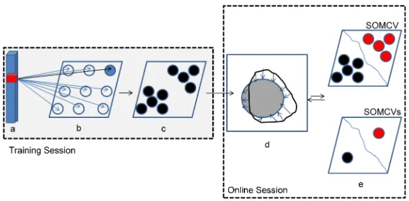
Fig. 1 illustrates the off-line and on-line components of theSOM CV andSOM CVsmodels in a vector-valued (more specifically,RGB) image segmentation framework (the scalar case is similar, but uses scalar pro-totypes and preferably a1-Dgrid). Fig. 1(a) shows the input layer of theSOM, whose dimension is equal to the one of the voxel intensities of the image to be segmented. For example, in the case ofRGBimages, the input layer of the map has dimension3, since it receives theR,G, andBchannels of the vector-valued image. The red cube in Fig. 1(a) represents a voxel intensity presented as input to theSOM, in this case made up of 3×3neurons (Fig. 1(b)). The small circles in Fig. 1(b) represent the neurons of the map, where each neuron is
associated with a three-dimensional prototype, of the same dimension as the input. The prototypes of the neurons
are modified during the training phase. This is accomplished by finding the best-matching neuron (the blue circle
in Fig. 1(b)) to each input voxel intensity, and updating its prototype and the ones of all its neighbors as described
in formulas (6), (7), (8), and (9), extended to the three-dimensional case as described in Subsection 4.2. Once
the learning is accomplished, the prototypes associated with selected neurons of the learned map (Fig. 1(b)) are
ready to be integrated into the energy functional (14) during the on-line session (i.e., during the curve evolution
process) as global regional intensity descriptors. Fig. 1(d) represents a test image to be segmented (the gray circle
represents the foreground). Starting from an initial contour (the black curve in Fig. 1(d)), the mean intensities of
inside and outside the contour are presented as inputs to the learned map in Fig. 1(c) to classify (see Fig. 1(e),
top) the prototypes associated with the neurons into foreground (in red) and background (in black) global
inten-sity descriptors. Then, the contour evolution is guided by the extracted prototypes associated with the two sets of
foreground and background neurons. In the case ofSOM CVs(see Fig. 1(e), down), only one prototype is used as a global intensity descriptor for each region.
5 Experimental study
In this section, we demonstrate the effectiveness and robustness of theSOM CV andSOM CVsmodels, com-pared to theC-V model described in Section 2, in handling real and synthetic images. For a fair comparison, the
Training Session
Online Session
a b c
d
e
Fig. 1: The architecture ofSOM CV forRGBimages: (a) the input intensities of a training voxel; (b) a3×3
SOM neural map (with a three-dimensional prototype associated with each neuron); (c) the trainedSOM; (d) the contour evolution process; and (e) the foreground (in red) and background (in black) representative neurons for theSOM CV (top) and theSOM CVs(down) models. For a scalar-valued image, a similar model is used, but the prototypes have dimension1, and a1-Dgrid is used.
PC with the following configuration: 2.5 GHz Intel(R) Core(TM) 2 Duo, and 2.00 GB RAM5. In each experiment,
ther0andσparameters are expressed in pixels. Moreover, theSOM CV andSOM CVsparameters are fixed6 as follows:η0=.9,σ= 1.5, and the weight parameters (i.e.,λ+,λ−for the scalar-valued case, andλ+i ,λ−i in the vector-valued case) are fixed to 1. Also,r0:= max(M, N)/2, whereMandNare the numbers of rows and columns of the installed neural map,t(tr)max = 10000,t(evol)max = 1000,τη :=t(tr)max,τr:= t(tr)max/ln(r0),ρ= 1.
For the experiments performed on the scalar-valued images considered in the paper, theSOMnetwork has been chosen as a1-Dneural map composed of5neurons (i.e.,M = 5andN = 1), whereas for the case of vector-valued images, it was a3×3grid of neurons in most experiments (M =N= 3) and a2×2grid (M =N = 2) for the other experiments (see Tables 3 and 4). In theC-V model,λ+,λ−for the scalar-valued case andλ+i ,
λ−i in the vector-valued case are also fixed to 1,µis chosen such that the final contour is smooth enough and
ν = 0(as made in [15, p. 268]). Moreover, theSOM CVsmodel is considered in the comparison with the same parameters of theSOM CV model. Unless stated otherwise, the training image used in the unsupervised train-ing session coincides with the test image. Otherwise, it is an image similar to the test image (obtained, e.g., by
adding Gaussian noise). In all the testing sessions, the initial contour has been chosen as rectangular. For the case
of gray-level images, the range of the values assumed by the intensity is 0-255 as all the considered gray-level
images are 8-bit images.
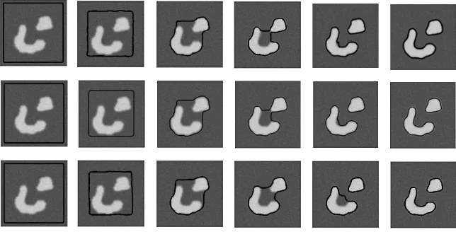
Fig. 2 shows the fast convergence ofSOM CV (and its variationSOM CVs) for scalar-valued images and the associated contour evolution process when compared to theC-V model. As Fig. 2 shows, the contours obtained by theSOM CV andSOM CVsmodels have converged to the respective final contours with similar numbers of performed iterations and similar performances because of the large intensity homogeneity of the image considered
in the experiment.
Fig. 3 illustrates the effectiveness and robustness with respect to noise ofSOM CV in handling images containing objects characterized by many different intensities and skewness/multimodality of the foreground
intensity distribution. The figure also compares the proposedSOM CV model with other unsupervisedACMs.
5 The developed code is available athttp://mohammedabdelsamea.weebly.com.
Fig. 2: The rapid contour evolution of theSOM CV andSOM CVsmodels when compared to the contour evolution of theC-Vmodel, in the scalar case. The first and second rows show, respectively, the contour evolution ofSOM CV andSOM CVs. From left to right: initial contour (in black), contour after 3, 6, 9, 12 iterations, and final contour (15 iterations). The third row shows the contour evolution of theC-V model. From left to right: initial contour (in black), contour after 50, 100, 150, 200 iterations, and final contour (260 iterations).
In particular, as compared to theC-V model, theSOM CV model has shown better results, due to its automated ability to preserve the topological structure of the foreground intensity distribution (this is not needed, instead, for
the background distribution, which is simpler). Moreover, Fig. 3 also compares the proposedSOM CV model to the unsupervisedSOM-basedACM7recently proposed in [24], which relies on both local and global intensity information with the aim of improving the robustness to the contour initialization. As demonstrated in Fig. 3,
SOM CV has been able to find better the objects and their boundaries. Finally, the segmentation performance of theSOM CVsmodel is quite similar to the one of theSOM CV model, but is also more sensitive to the noise.
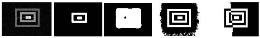
a
b
Fig. 3: The effectiveness of theSOM CV model in dealing with objects characterized by many different intensi-ties and skewness/multimodality of the foreground intensity distribution. Arranged in rows there are: (a) a noisy 140×100image (with Gaussian noise added, standard deviationSD = 10) with six different intensities 80, 100, 140, 170, 200, and 230 in its foreground; (b) a noisy90×122image (with Gaussian noise added, standard deviationSD= 10) with three different intensities 100, 150, and 200 in its foreground. The columns from left to right show: the images with the additions of the initial contours, the histograms of the intensities of the images, and, respectively, the segmentation results of theSOM CV model and theSOM CVsmodel (σ =.5,1.5have been used, respectively, for (a) and (b)), of theC-V model, and of the model proposed in [24].
7 Since in the paper we are interested in unsupervisedACMs, we have not compared the proposedSOM CV model to the
As a motivating example for the development of the proposedSOM CV model, Fig. 4 shows the behavior of several other unsupervisedACMs from different classes, which have been tested on the image of Fig. 3 (second row), providing unsatisfactory segmentation results. As illustrated in Fig. 4, the model proposed in [29] - which
is an unsupervised globalACM based on the means of sign pressure forces, and relies on strong statistical as-sumptions - has failed in finding properly the foreground. Similarly, the boundary-based active contour model
from [30] - whose energy functional includes a Laplacian image term - has failed in segmenting the same image.
Also the models of [31] and [32] - which are localACMs (i.e., they do not take into account spatial dependen-cies among the pixels) - have shown unsatisfactory results, possibly due to the high sensitivity to the contour
intialization and noise, which is typical of localACMs.
Fig. 4: The segmentation results obtained by some well-known unsupervisedACMs on the image of Fig. 3 (second row). From left to right: the original image with the initial contour, and the segmentation results obtained by the unsupervisedACMs proposed in [29], [30], [31], and [32], respectively.
Then, in order to demonstrate the robustness ofSOM CV andSOM CVsto the additive noise, in the ex-periment described in Fig. 5 we have used the top left image of Fig. 3 in the training session ofSOM CV and
SOM CVs, then the trainedSOM (whose values of the weights are commom to the two models) has been ap-plied on-line to various test images obtained adding to such an image different levels of Gaussian noise. As shown
in Fig. 5, for this caseSOM CV is more robust and less sensitive to the additive noise thanSOM CVs, since the regions of the foreground are detected more accurately bySOM CV.
Similarly, the image of Fig. 3(b) has been used in the training session ofSOM CV andSOM CVs, then the trainedSOM has been applied on-line to various test images obtained by adding to such an image different levels of Gaussian noise, as shown in Fig. 6. The results of these two experiments show the ability ofSOM CV
to find all the different regions of the object (which is characterized by many different intensities), and also its
robustness to the additive noise and to the skewness/multimodality of the foreground intensity distribution. They
also demonstrate that, in the case of images containing objects characterized by many different intensities or by
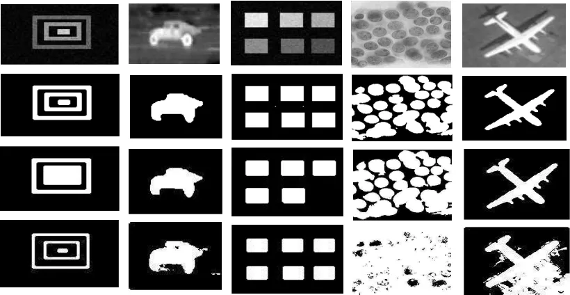
skewed/multimodal intensity distributions,SOM CV is expected to produce better results thanSOM CVs. Fig. 7 illustrates the effectiveness ofSOM CV in handling real and synthetic scalar-valued images. The segmentation results of theSOM CV model on the real images shown in the first and second columns show the ability ofSOM CV to segment objects with blurred edges and background, while theC-V model provides a worse segmentation for the image in the first column, and incurs in an under-segmentation problem for the image
in the second column. Similarly,SOM CV outperformsC-V also in handling synthetic images as shown in the third and fourth columns. Moreover, SOM CV andSOM CVsbehave exactly the same asC-V in handling binary gray images as in the case of the image shown in the right-most column. This is because in this case the
mean intensities inside and outside the contour are accurate enough to approximate the foreground/background
Fig. 5: The robustness of theSOM CV andSOM CVsmodels to the additive noise: the first row shows, from left to right, the image of Fig. 3(a) with the addition of different Gaussian noise levels (standard deviationSD= 10, 15, 20, and 25, respectively); the second and third rows show, respectively, the corresponding segmentation results ofSOM CV andSOM CVs.
Fig. 6: The robustness of theSOM CV andSOM CVsmodels to the additive noise: the first row shows, from left to right, the image of Fig. 3(b) with the addition of different Gaussian noise levels (standard deviationSD= 10, 20, 30, 40, and 50, respectively); the second and third rows show, respectively, the corresponding segmentation results ofSOM CV andSOM CVs.
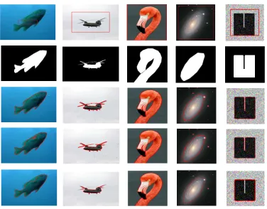
To illustrate the effectiveness ofSOM CV and its variationSOM CVsin handling real and synthetic vector-valued images, we have tested the extension ofSOM CV andSOM CVsto the vectorial framework onRGB
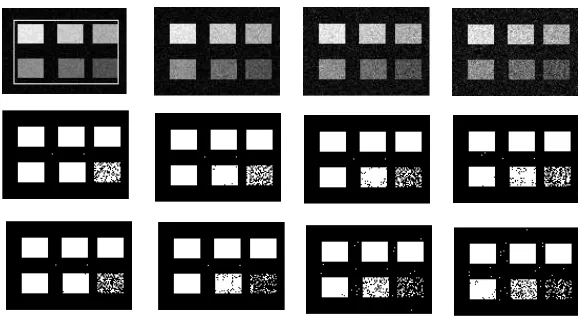
real and synthetic images, which is shown in Fig. 8 in comparison with the vectorialC-V model from [15]. The segmentation results ofSOM CV are similar to the ones ofC-V in handling the image shown in the fourth col-umn, whileSOM CV outperformsC-V in all the other shown images. For these images,SOM CV outperforms alsoSOM CVs, which, however, provides better results thanC-V, apart from the cases of the images considered in the first two columns, for which the results are similar.
In the following, we provide also a quantitative study to confirm the effectiveness ofSOM CV andSOM CVs, when compared toC-V. To demonstrate quantitatively the accuracy of theSOM CV andSOM CVsmodels in segmenting the images shown in Fig. 7 and 8, we have also compared the obtained segmentation results with
their corresponding ground-truth data by adopting the Precision (P), Recall (R), andF-measure metrics. They are defined as follows:
Precision(P) := T P
Fig. 7: The segmentation results obtained on real and synthetic scalar-valued images. The first, second and third row show the original images with the initial contours, the histograms of the image intensities and their ground truth, respectively, while the fourth, fifth, and sixth rows show, respectively, the corresponding segmentation results of theSOM CV,SOM CVsandC-V models.
Recall(R) := T P
T P+F N, (31)
F-measure(F-m) := 2P R
P +R, (32)
whereT P,F P, andF N represent, respectively, the numbers of true positive, false positive, and false negative foreground pixels. Precision and Recall are sensitive to the amount of over-segmentation and under-segmentation,
respectively, in the sense that over-segmentation is associated with a small Precision score, whereas
under-segmentation leads to a small Recall score. Finally, theF-measure quantifies the overall accuracy.
Tables 1 and 2 illustrate the high segmentation accuracy of theSOM CV model and its variationSOM CVs
when compared to theC-V model, in terms of the three metrics defined above. As the two tables illustrate, the
Fig. 8: The segmentation results on real images from [33, 34], and synthetic vector-valued images. The first and second rows show the original images with the initial contours, respectively, while the third, fourth, and fifth rows show, respectively, the corresponding segmentation results of the vectorial versions of theSOM CV,SOM CVs
andC-V models. Note thatσ = .5has been used bySOM CV andSOM CVsfor the image in the second column.
Table 1: The Precision, Recall, andF-measure metrics for the scalarSOM CV,SOM CVsandC-V models in the segmentation of the scalar images shown in Fig. 7.
Image in SOM CV SOM CVs C-V
P(%) R(%) F-m (%) P(%) R(%) F-m (%) P(%) R(%) F-m (%)
column 1 98.8 99.9 99.3 75.5 100 86 91.8 83.3 87.4
column 2 60.6 98.5 75 60.6 98.5 75 42.7 98.5 59.6
column 3 100 100 100 100 100 100 99.2 88 93.3
column 4 96.3 99.3 97.8 98.8 98.4 98.6 96.5 96.4 96.4
column 5 100 100 100 100 100 100 99 100 99.5
Table 2: The Precision, Recall, andF-measure metrics for the vectorialSOM CV,SOM CVsandC-V models in the segmentation of theRGBimages shown in Fig. 8.
Image in SOM CV SOM CVs C-V
P(%) R(%) F-m. (%) P(%) R(%) F-m. (%) P(%) R(%) F-m. (%)
column 1 89.6 96.8 93 91.3 91.8 91.5 94.7 83.1 88.5
column 2 71.7 97.6 82.7 72.3 97.3 82.9 84.5 81.9 83.2
column 3 94.4 90.1 92.2 95 89 91.9 89.5 88.9 89.2
column 4 96.1 85.5 90.5 93.5 91.7 92.6 96.1 86.9 91.3
column 5 99.6 100 99.8 100 100 100 96.8 89.6 93.1
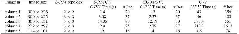
To demonstrate the computational efficiency of theSOM CV andSOM CVsmodels when compared to the
C-V model, Table 3 shows, for each of the three methods, theCP Utime (in seconds) that was required for the contour evolution (i.e., the time required in the testing session) and the number of iterations performed before
Moreover, the computational effectiveness of the vectorial versions ofSOM CV andSOM CVswith respect to the vectorialC-V model is illustrated in Table 4 for theRGBimages in Fig. 8 by showing, for all methods, theCP U times and the number of iterations required in the testing session (note that, in the common training session ofSOM CV andSOM CVs, theCP Utime is fixed by the number of iterationst(tr)max). The sizes of the
training and test scalar-valued and vector-valued images are also listed in the two tables. From these tables, we
can observe that theSOM CV andSOM CVs models were much faster than theC-V model in all the listed cases, as the contour evolution forSOM CV andSOM CVsrequired less iterations to converge than for the
C-V model, and also the computational time per iteration for theSOM CV andSOM CVsmodels was smaller than the one for the C-V model. This is due to the fact that SOM CV andSOM CVs models are Gaussian Regularizing Level Set Models, whereas the originalC-V model has not this feature.
Concluding, the results shown in Tables 1-4 highlight several advantages of theSOM CV andSOM CVs
models with respect to theC-V model.
Table 3: The contour evolution time and number of iterations required by theSOM CV,SOM CVs, andC-V
models to segment the foreground for the scalar-valued images shown in Fig. 7.
Image in Image size SOMtopology SOM CV SOM CVs C-V
CP UTime (s) # Iter. CP UTime (s) # Iter. CP UTime (s) # Iter.
column 1 118×93 5×1 0.03 10 0.01 9 6.22 137
column 2 256×256 5×1 1.0 30 0.73 30 104.2 406
column 3 114×101 5×1 0.14 16 0.1 16 5.6 100
column 4 135×125 5×1 0.15 16 0.15 16 13.1 266
column 5 64×61 5×1 0.03 7 .01 7 4.38 97
Table 4: The contour evolution time and number of iterations required by theSOM CV,SOM CVs, andC-V
models to segment the foreground for the vector-valued images shown in Fig. 8.
Image in Image size SOMtopology SOM CV SOM CVs C-V
CP UTime (s) # Iter. CP UTime (s) # Iter. CP UTime (s) # Iter.
column 1 300×225 2×2 1.4 20 1.2 20 43 356
column 2 300×225 3×3 3.08 37 2.57 37 46 400
column 3 300×451 3×3 14.35 80 12.19 80 588.4 551
column 4 272×297 3×3 2.9 25 2.79 27 212.3 1612
column 5 114×101 2×2 .9 16 .4 16 4.6 78
In the following experiments, for a fair comparison, we compare the behavior of ourSOM CV model, as a
variational level set-basedSOM-basedACM, with theCSOM CV model [11] and the Local-GlobalSOM
-basedACMfrom [24], as related state-of-the-art variational level set-basedSOM-basedACMs. Moreover, we
also include in the comparison theSOM-based Hierarchical Agglomerative Clustering (SOM-HAC) model
from [35], as a SOM-based - but not variational level set-based - image segmentation model. SOM-HAC
relies on local features (including, for each pixel, its local mean intensity and standard deviation), which are used
in a first stage as inputs to train aSOM. Then, in a second phase, it makes use of hierarchical agglomerative
clustering to perform an additional clustering process of the output prototypes of theSOM, hence producing the
final segmentation.
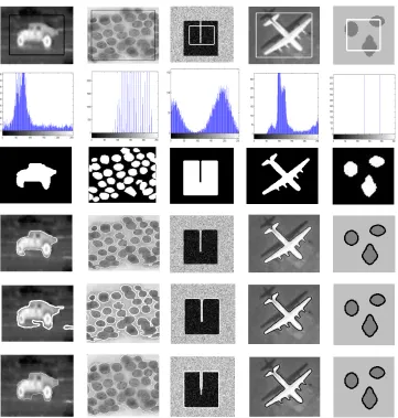
Fig. 9 shows, for some of the scalar-valued images presented in the paper, a comparison of the segmentation
ACM), and theSOM-HACmodel (as a localSOM-based segmentation model). Fig. 11 also shows the choice
of the supervised pixels for theCSOM CV model. As illustrated in Fig. 9,SOM CV has shown a significant
performance in segmenting such images, often outperforming such state-of-the-artSOM-based models and, in
the other cases, showing at least similar results. Moreover, both its effectiveness and efficiency have been
con-firmed by the quantitative results reported in Tables 5 and 6, respectively. As compared to theCP U time of
SOM CV, the one ofCSOM CV is sometimes slightly smaller, sinceCSOM CV uses a scalar value to
repre-sent an intensity distribution, while the proposedSOM CV model uses a set of descriptors for its representation.
However, this slighlty larger computational effort makes it possible to obtained better final segmentations, despite
beingSOM CV an unsupervised model.
Finally, Table 7 reports theCP Utime and the associated number of iterations required by the unsupervised
SOM-basedACM presented in [24] (as a Local-GlobalSOM-based ACM) to produce, on the last three
images of Fig. 7, similar segmentation results as theSOM CV andSOM CVs models (such segmentations
are shown in Fig. 10). The table highlights the larger efficiency of theSOM CV andSOM CVsmodels when
compared to the model from [24]. The largerCP Utimes of the latter are due to the fact that it uses both local
and global information in each iteration, during the evolution of its active contour.
Fig. 9:The binary segmentation results of our proposedSOM CV model, as compared to theCSOM CV and SOM-HACmodels. The first row shows the original images. The second row shows the segmentation results, corresponding to the images in the first row, obtained by theSOM CVmodel. The third and fourth rows show the corresponding binary segmentation results obtained by theCSOM CV andSOM-HACmodels, respectively.
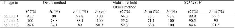
In order to compare ourSOM CV model with some representative global pixel-based segmentation tech-niques, we have applied the Otsu’s method [36] and the multi-threshold Otsu’s method [37] to some of the
scalar-valued images considered in this paper. Such methods belong to the class of thresholding image segmentation
methods, as they segment a scalar-valued image by comparing the pixel intensity with one or multiple thresholds,
respectively. The main reason for selecting the Otsu’s method is that its threshold is chosen in such a way to
Fig. 10:The segmentation results obtained by the unsupervisedSOM-basedACM proposed in [24] on some of the images presented in Fig. 7.
Fig. 11:The training images used by theCSOM CV model together with the supervised foreground pixels (red) and the supervised background pixels (blue) used in the training sessions of the model.
Table 5:The Precision, Recall, and F-measure metrics for theCSOM CV andSOM-HAC methods in the segmentation of the images shown in Fig. 9, as compared to theSOM CV model.
Image in SOM CV CSOM CV SOM-HAC
P(%) R(%) F-m (%) P(%) R(%) F-m (%) P(%) R(%) F-m (%)
column 1 100 84.4 91.5 77.4 69 73 100 39.6 56.7
column 2 98.8 99.9 99.3 100 78 87 89.9 80.7 85.1
column 3 100 90.5 95 100 74.6 85.4 100 100 100
column 4 60.6 98.5 75 92 86.6 89.2 45.2 69.4 54.8
column 5 96.3 99.3 97.8 78.3 81.3 79.8 24.3 78.1 37
Table 6:The contour evolution time and number of iterations required by theSOM CV model as compared to the CSOM CV model to segment the foreground for some of the scalar-valued images shown in Fig. 9, in addition to the convergence time required by theSOM-HACmodel, for the same images.
Image in SOM CV CSOM CV SOM-HAC
CP UTime (s) # Iterations CP UTime (s) # Iterations CP UTime (s)
column 1 0.03 10 .03 8 2.65
column 2 0.05 10 0.04 10 3.9
column 3 0.35 14 0.3 12 3.1
column 4 4.06 32 2.1 32 9.25
column 5 0.92 17 0.32 16 5.5
Table 7:The contour evolution time and number of iterations required by the unsupervised ACM proposed in [24] to segment the foreground for some of the scalar-valued images shown in Fig. 7, as compared to the contour evolution time and number of iterations required by theSOM CV andSOM CVsmodels, for the same
images.
Image in SOM CV SOM CVs Model in [24]
CP UTime (s) # Iterations CP UTime (s) # Iterations CP UTime (s) # Iterations
column 3 0.14 16 0.1 16 12.15 30
column 4 0.15 16 0.15 16 15.19 16
column 5 0.03 7 .01 7 .45 7
the foreground and the background, respectively) and the minimization of the intra-class variance (i.e., between
pairs of pixels belonging to the same region). The multi-threshold the Otsu’s method is similar but uses more
thresholds, segmenting the image in more than2regions. Fig. 12 shows the segmentation results obtained by
the Otsu’s method (second row) and the multi-threshold Otsu’s method (third row) on some of the scalar-valued
merged some of the objects found for different numbers of thresholds (as shown in the fourth row), then we have
applied the classical Otsu’s method to the resulting image (fifth row). As illustrated by Fig. 12, the Otsu’s and
multi-threshold Otsu’s methods demonstrated to be more sensitive to noise than our proposedSOM CV model. As an additional drawback, post-processing operations were also required for the multi-threshold Otsu’s method.
The quantitative results corresponding to Fig. 12 are reported in Table 8.
Table 8: The Precision, Recall, andF-measure metrics for the Otsu’s method and the multi-threshold Otsu’s method (with post-processing) in the segmentation of the images shown in Fig. 12 (second and fifth rows, respec-tively) compared to theSOM CV model (sixth row).
Image in Otsu’s method Multi-threshold SOM CV
Otsu’s method
P(%) R(%) F-m (%) P(%) R(%) F-m (%) P(%) R(%) F-m (%)
column 1 97.7 98 97.8 100 64.3 78.3 98.8 99.9 99.3
column 2 100 78.8 88.1 100 55.2 71.1 100 90.5 95
column 3 94.4 84.1 89 98.7 52.3 68.4 100 84.4 91.5
Finally, we have trained the neural map on a single frame of a real aircraft video [38] (the top left image in
Fig. 13(a)) and applied the trained network on-line to segment individually - usingSOM CV - some of itsRGB frames, which are shown in Fig. 13(a) (the initial contours for the video frames are similar to the initial contour
-shown in red - which has been used for the first image). Fig. 13(b) shows the segmentation results ofSOM CV in handling the selected frames in Fig. 13(a) and demonstrates its robustness to scene changes and object motions.
Concluding, this experiment hightlights the robustness ofSOM CV model to the contour initialization, scene changes and illumination variations when being used in an on-line framework.
6 Discussion
Unsupervised globalACMs are powerful segmentation techniques which are able to segment images in an unsu-pervised global way by dealing with the segmentation process as an optimization problem. However, a limitation
of existing unsupervised globalACMs is in the statistical assumptions made on the image intensity distribution. Motivated by the above observation, we have proposed a novel unsupervised globalACM, termed SOM-based Chan-Vese(SOM CV). The SOM CV model is a global and an unsupervised ACM that integrates effectively the advantages ofACMs and self-organizing networks.SOM CV has aSelf-Organizing Topology Preservation(SOT P) property, which allows to preserve the topological structures of the foreground/background intensity distributions during the active contour evolution. Indeed,SOM CV relies on a set of self-organized neu-rons by automatically extracting the prototypes of selected neuneu-rons as global regional descriptors and iteratively,
in an unsupervised way, integrates them during the evolution of the contour.
In order to highlight the robustness ofSOM CV, several synthetic and real images with different kinds of intensity distributions have been handled effectively in the experimental studies presented in Section 5. Also
the variation ofSOM CV - theSOM CVsmodel - has provided good results in most cases. The capability of
Fig. 12: The segmentation results of the Otsu’s and the multi-threshold Otsu’s methods on some of the scalar-valued images considered in this paper. The first row shows the original images. The second row shows the segmentation results, corresponding to the images of the first row, obtained by the Otsu’s method. The third row shows the object of interests obtained by the multi-threshold Otsu’s method when the number of thresholds is five. The fourth row shows the merged objects obtained by first applying the multi-Otsu’s method when the number of thresholds is 2, 3, 4, and 5, then merging some of the obtained objects. The fifth row shows the segmentation results of the Otsu’s method applied on the images of the fourth row. Finally, the sixth row shows the segmentation results obtained bySOM CV on the images of the first row.
The following are some possible directions for future developments. The first one consists in extending the
SOM CV andSOM CVsmodels such that the underlying neurons are incrementally added/removed and trained to overcome the limitation of manually adapting the topology of the network. Moreover, one may apply suitable
tools (e.g., genetic algorithms) to identify the bestSOM topology, thus reducing the number of parameters to be tuned manually. Furthermore, one may use both local and global information to enableSOM CV and
SOM CVsto handle, still in a robust and unsupervised way, images with larger intensity inhomogeneity of the foreground/background and more complex intensity distributions.
Compliance with Ethical Standards
b a
Fig. 13: The robustness of theSOM CV model to scene changes and moving objects. (a) The first row shows the original early frames (frames 50-59, from left to right) of a real-aircraft video while later frames (frames 350-359, from left to right) are shown in the second row. (b) shows the segmentation results obtained bySOM CV, on the frames shown in part (a).
References
1. Y. V. Venkatesh, S. Kumar Raja, N. Ramya, A novel SOM-based approach for active contour modeling, in: Proceedings of the
2004 Conference on Intelligent Sensors, Sensor Networks and Information Processing, 2004, pp. 229–234.
2. C. Xu, J. L. Prince, Snakes, shapes, and gradient vector flow, IEEE Transactions on Image Processing 7 (3) (1998) 359–369.
3. T. F. Chan, L. A. Vese, Active contours without edges, IEEE Transactions on Image Processing 10 (2) (2001) 266–277.
4. M. F. Talu, ORACM: Online region-based active contour model, Expert Systems with Applications 40 (16) (2013) 6233 – 6240.
5. M. M. Abdelsamea, S. A. Tsaftaris, Active contour model driven by globally signed region pressure force, in: Proceedings of the
18th International Conference On Digital Signal Processing, 2013.
6. S. Chen, R. J. Radke, Level set segmentation with both shape and intensity priors, in: Proceedings of the 12th IEEE International
Conference on Computer Vision, 2009, pp. 763–770.
7. T. Kohonen, Essentials of the self-organizing map, Neural Networks 37 (2013) 52–65.
8. S. R. Vantaram, E. Saber, Survey of contemporary trends in color image segmentation, Journal of Electronic Imaging 21 (4),
article ID: 040901, 28 pages, 2012.
9. S. Skakun, A neural network approach to flood mapping using satellite imagery, Computing and Informatics 29 (6) (2010) 1013–
1024.
10. M. M. Abdelsamea, G. Gnecco, M. M. Gaber, A survey of SOM-based active contours for image segmentation, in: Proceedings of
the 10th Workshop on Self-Organizing Maps (WSOM 2014), Advances in Intelligent Systems and Computing, Vol. 295, Springer,
2014, pp. 293–302.
11. M. M. Abdelsamea, G. Gnecco, M. M. Gaber, A concurrent SOM-based Chan-Vese model for image segmentation, in:
Proceed-ings of the 10th Workshop on Self-Organizing Maps (WSOM 2014), Advances in Intelligent Systems and Computing, Vol. 295,
Springer, 2014, pp. 199–208.
12. M. M. Abdelsamea, G. Gnecco, M. M. Gaber, An efficient self-organizing active contour model for image segmentation,
Neuro-computing 149, Part B (2015) 820–835.
13. D. Mumford, J. Shah, Optimal approximations by piecewise smooth functions and associated variational problems,
Communica-tions on Pure and Applied Mathematics 42 (5) (1989) 577–685.
14. H.-K. Zhao, T. Chan, B. Merriman, S. Osher, A variational level set approach to multiphase motion, Journal of Computational
![Table 7: The contour evolution time and number of iterations required by the unsupervised ACM proposedin [24] to segment the foreground for some of the scalar-valued images shown in Fig](https://thumb-us.123doks.com/thumbv2/123dok_us/1014886.1601440/22.596.146.421.99.179/contour-evolution-iterations-required-unsupervised-proposedin-segment-foreground.webp)