Rollout Algorithm Based Duty Cycle Control with
Joint Optimisation of Delay and Energy Efficiency
for Beacon-enabled IEEE 802.15.4 Networks
Yun Li, Kok Keong Chai, Yue Chen
School of Electronic Engineering and Computer Science Queen Mary University of London
Email:{yun.li, michael.chai, yue.chen}@qmul.ac.uk.
Jonathan Loo
Department of Computer and Communications Engineering Middlesex University
Email: [email protected]
Abstract—Duty cycle control is applied in IEEE 802.15.4 medium access control (MAC) protocol to reduce energy con-sumption. A low duty cycle improves the energy efficiency but it reduces the available transmission time, thereby increases the end-to-end delay. Thus, it is a challenge issue to achieve a good trade-off between energy efficiency and delay. In this paper, we study a duty cycle control problem with the aim of minimising the joint-cost of energy consumption and end-to-end delay. By applying dynamic programming (DP), the optimal duty cycle control is derived. Furthermore, to ensure the feasibility of implementing the control on computation limited sensor devices, a low complexity rollout algorithm based duty cycle control (RADutyCon) is proposed. The joint-cost upper bound of the proposed RADutyCon is investigated. Simulation results show that RADutyCon can effectively reduces the joint-cost of energy consumption and end-to-end delay under various network traffic. In addition, RADutyCon achieves an exponential reduction of computation complexity compared with DP optimal control.
I. INTRODUCTION
The emerging wireless sensor and actor networks (WSANs) are featured as integrating various applications and providing device-varied data delivery in terms of energy efficiency and end-to-end delay [1], [2]. IEEE 802.15.4 standard [3] utilises low duty cycle to conserve energy by putting devices into inac-tive mode. However, a lower duty cycle introduces higher end-to-end delay due to the reduced available transmission time. In addition, as application requirements various from device to device, the uniformed duty cycle control for all devices in current standard may not provide the best overall performance to meet the requirement for applications in WSANs.
The idea of achieving a trade-off between energy efficiency and end-to-end delay through adaptive duty cycle control of MAC protocols was explored by Dynamic Sensor MAC pro-tocol (DSMAC) [4]. In DSMAC, duty cycle is adjusted based on the threshold of energy utilisation efficiency and average latency experienced by the sensor. However, the duty cycle adaptation of DSMAC can only be double or half of the initial setting. The delay reduction of U-MAC [5] is achieved by controlling the length of active periods based on a utilisation function, which is the ratio of the actual transmission and receptions performed by the device. However, the uniformed duty cycle control for all devices is not flexible when each
device generates different amount of traffic with different quality of service (QoS) requirements. The duty cycle control algorithm called Traffic-adaptive Distance-based Duty Cycle Assignment (TDDCA) is proposed in [6], with the aim of meeting a target transmission rate while minimising the energy consumption. The duty cycle is increased when contention is reported. Otherwise, the duty cycle is decreased every time period down to a minimum. However, to enable the control, contention reports, piggyback flags and modifications of the packet header are needed. In [7], DutyCon is proposed to guarantee end-to-end delay by assigning a local delay require-ment to each single hop along the communication flow. In this method, a feedback controller is designed to adapt the sleep interval to meet the single-hop delay requirement. However, this approach requires significant amount of signalling from the neighbour devices to compute the delay. To reduce the signalling among neighbour devices, a distributed duty cycle controller is proposed in [2] aiming at controlling the local queue length of the device to be the same as the predetermined threshold. The distributed duty cycle control is achieved by adjusting the sleep duration of each device based on its local queue length independently. However, this approach needs specific syntonisation scheme, and the evolution of the proposed control requires carefully setting of the initial duty cycle and control parameters.
While the aforementioned literatures laid a solid founda-tion in designing adaptive duty-cycled MAC protocols, less work has been done in terms of the duty cycle optimisation with joint consideration of energy consumption and end-to-end delay. To address the above joint consideration, in this paper we study an optimisation problem aiming at minimising energy consumption and end-to-end delay jointly. A joint-cost function, which follows a similar logic of the joint consideration of purchase cost and store cost in inventory control problem [8], is designed as the weighted sum of energy consumption and end-to-end delay. The weighting factors of the joint-cost function are adjustable according to different requirements on energy consumption and end-to-end delay of each device or specific application requirements.
first, we formulate an optimisation problem to minimise the joint-cost, taking the network traffic and the device position into consideration. Then, the optimal duty cycle control is derived by applying dynamic programming (DP). Furthermore, a rollout algorithm based control (RADutyCon) is proposed to reduce the computation complexity of running DP on sensor devices. In addition, the joint-cost upper bound of the proposed RADutyCon is investigated.
The remainder of the paper is organised as follows. In section II, we give the system model and the background of IEEE 802.15.4 MAC protocol. Problem formulation is given in Section III. Section IV presents the derived optimal solution and the proposed RADutyCon. Simulation results and conclusion are given in section V and section VI, respectively.
II. SYSTEMMODEL
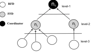
Among the different multi-hop WSANs, the simple two-hop cluster-tree network model has been the focus of much ongoing research. This paper dedicated to the analysis of two-hop cluster-tree network while the multi-hop case can be viewed as the combination of several two-hop scenarios. We consider a three-level cluster-tree network as shown in Fig. 1. The coordinator n0 is in level-1; the full-function devices
(FFDs/actors)ni (1≤i≤N) are in level-2 and the
reduced-function devices (RFDs/sensors) are in level-3. The level of the device is denoted aslni, in particular, ln0 = 1. FFDs can communicate with the coordinator and its child RFDs, whereas RFDs can only communicate with its parent FFD.
n0
ni
RFD
FFD
Coordinator n
j level-1
level-2
level-3
Fig. 1. Network Model.
A. IEEE 802.15.4 (2011)
We adopt IEEE 802.15.4 (2011) beacon-enabled mode where each FFD periodically broadcasts the beacon to its child devices. The duration between two consecutive beacons is called Beacon Interval (BI), while the duration of an active period is called Superframe Duration (SD). Specifically,
BI=aBaseSuperF rameDuration×2BO, (1) SD=aBaseSuperF rameDuration×2SO, (2) where Beacon Order (BO) and Superframe Order (SO) are two integers ranging from 0 to 14 (0≤SO≤BO≤14), and aBaseSuperF rameDuration= 15.36ms at 2.4 GHz with 250 kbps bandwidth. The duty cycle is defined as the ratio of the active portion over each time period, thus
Duty Cycle=SD/BI= 2SO−BO. (3)
In multi-hop transmission, each FFD divides its BI into two superframes, named incoming superframe and outgoing superframe, as shown in Fig. 2. The FFD ni receives the
beacon from the coordinator in the incoming superframe, and transmits its beacon in the outgoing superframe. As there are twoSDsin eachBI, according to (1) and (2),SO≤BO−1 for all FFDs. Theoretically speaking, the duty cycle of different devices could be different, but in the current standard they are all equal [3].
Fig. 2. Superframe structure of IEEE 802.15.4.
To simplify the problem, we aim at controlling the out going superframe duty cycle (refer as duty cycle in this paper) of the FFDs. The incoming superframe duty cycle is decided by the parent FFD of the device and enclosed in the received beacon. We set all devices to be activated at the beginning of eachBI. The same BO is set to all devices in the network with the aim of simplifying the synchronisation. Thus, the duty cycle control of each FFD is achieved by setting the outgoing SO based on the number of packets generated by its child devices.
B. Queue and Traffic Models
We assume all generated packets are available at the be-ginning of each time period. All the packets are forwarded to the coordinator n0 for uplink transmission and qnmaxi is the maximum queue length of the device ni. The new arrived
packets will be dropped if the queue length in the buffer reaches its maximum. Similar to [5], the queue length of time period k+ 1 of device ni is given as
qnk+1i = min
[qkni+rnki−fnki+gnki]+, qnmaxi
, (4)
where0≤k≤K−1,[·]+= max(0,·),gk
ni is the number of packets being generated by device niin time period k;fnki is the number of packet transmited by deviceni in time period
k; and rk
ni is the number of packets received by device ni in time period k. Note that rkni equals to zero if device ni
has no child device. We assume the number of packets each device sends to its parent device follows Poisson distribution and each device generates a Poisson distributed integer number of packets in each time period (BI). Thus, fnki and g
k ni are independent random variables.
III. PROBLEMFORMULATION
minimize the total expected joint-cost of energy consumption and end-to-end delay.
To minimise the total expected joint-cost of energy con-sumption and end-to-end delay, we define the transmitting en-ergy consumption costEt(fnki), receiving energy consumption costEr(rkni), idle listening energy consumption costEl(r
k ni), and end-to-end delay cost D(rkni)of deviceni as
Er(rnki) =cr×
rk ni
qmax ni ×lni
(5)
Et(fnki) =cf×
fnki
qmax ni ×lni
, (6)
El(rnki) =cl× [fk
ni−g
k ni−q
k ni−r
k ni]
+
qmax ni ×lni
, (7)
D(rnki) =cd×
[qnki+rkni+gnki−fnki]+
qmax ni ×lni
, (8)
where cf, cr, cl and cd are the coefficients of transmitting,
receiving, idle listening and delay of the device, respectively. Note that cr < cl, as if cr were greater than cl, it would
never be optimal to receive new packets in the last period and possibly in earlier periods.
We further introduce α and β to assign the weightings of energy efficiency and end-to-end delay requirements of different applications. The expected weighted-sum joint-cost function for deviceni at time periodkis
J(rnki) =E
α
Ef(fnki) +Er(r
k
ni) +El(r
k ni)
+βD(rnki)
.
(9)
where3α+β = 1, as there are three terms using the weighing factorα.
We adopt IEEE 802.15.4 (2011) standard, which applies slotted carrier-sense multiple access with slotted collision avoidance (CSMA/CA) for packet transmission. Before the packet transmission, we assume devices need to perform two clear channel accesses (CCAs). Within each superframe dura-tion, the beacon transmission duration isDbcn. Thus, the total
packet transmission durationP D=SD−Dbcn. If
acknowl-edgement (ACK) is required for each packet, the successful packet transmission periodPs=dPCCA+PL+δ+PACKe,
wherePCCAis the transmission time for two CCAs,PLis the
transmission time for each packet, δ and PACK are waiting
and transmission time of the ACK packet, respectively. Hence, the number of packets that can be received by deviceniatkth
time periodrk
ni =P D/Ps.
Because of the collision, the transmission throughput is limited according to the number of contending devices. We adopt the throughput limitation coefficientb of [9]. Based on (2), the relationship betweenSO and the amount of packets the device could receive in time period kis given as follow
SOni(k) = &
log2(r
k ni×Ps
b +Dbcn)
'
. (10)
Our objective is to find the control of the optimal duty cycles πn∗i for each deviceni over K time periods, which minimise
the overall expected joint-cost. Hence, the joint optimisation problem is:
Pni : πmin ni∈D
E
(K−1
X
k=0
J(rnki) )
(11)
s.t. qKni = 0, rkn
i ≤r
max ni ,
where D is valid duty cycle sets of device ni and rnmaxi is the maximum number of packets device ni could receive.
According to (1)-(3), the range of D is restricted by the maximum valid SO.
IV. ADAPTIVEDUTYCYCLECONTROL
In this section, we first derive the optimal solution of prob-lem Pni. As the optimal solution is difficult or impractical to implement on computation-limited sensor devices, we further propose a low-complexity RADutyCon, and give its joint-cost upper bound.
A. Optimal Duty Cycle Control
By applying the principle of DP, the problem Pni is decomposed into a sequence of subproblems S(rnki), where 0 ≤k ≤K. The objective of each subproblem S(rkni)is to minimise the sum of joint-cost functions from time period k to K. Thus, the total cost ofPni is equal to that of S(r
0
ni), which means the optimal solution of S(r0
ni) is the optimal solution ofPni. Based on (9), the cost-to-go functionU(r
k ni) of S(rk
ni)is
U(rkni) = min
πni∈SE
α(Er(rkni) +Et(f
k
ni)) +H(r
k
ni) (12) +E{U(rnk+1i )}
,
whereH(rkni) =E
αEl(rnki) +βD(r
k ni)
shows the tradeoff
between idle listening energy consumption cost and the end-to-end delay cost. For simplicity, we introducemk
ni =q
k ni+r
k ni andnkni =fnki−gkni, combined with (7) and (8),H(rkni)can be rewritten as
H(mkni) =E
αcl×
max(qmax ni ,[n
k ni−m
k ni]
+
)
qmax×lni
(13)
+βcd×
max(qmax ni ,[m
k ni−n
k ni]
+
)
qmax×lni
.
As the convexity preserved by taking expectation overnk ni, with each fixednk
ni,H(m
k
ni)is convex. To take the convexity of H(mk
ni), we rewrite (12) as
U(mkni) = minπ ni∈S
E
W(mkni)−αcr×
qnki
qmax×lni
, (14)
where
W(mkn
i) =αcr×m
k
ni+αEt(f
k
ni) +H(m
k
ni) (15) +E
U([mkn+1i −q
k+1
ni ]
+))
Then the objective ofS(rkni)is to find the minimum value of (14). Based on (10) and (12)-(15), the optimal duty cycle control at each time period can be found by running DP.
Throrem 1:IfW(mk
ni)is convex, and
mkn
i ∗
=Tni = arg min
mk ni∈<
W(mkn
i), (16)
where<as the set of all valid values ofmk
ni. Then, the optimal solution ofPni is
SOkn
i ∗ =
log2(
rnik ∗×Ps
b +Dbcn)
if qni(k)< Tni,
dlog2(Dbcn)e if qni(k)≥Tni. (17)
Proof:Fork=K, functionU(mK
ni)is the zero function, so it is convex. Since cr < cd and the derivative ofH(mKni) tends to−cd/lni as q
K ni+r
K
ni→ −∞, thusW(m
K−1
ni )has a derivative that becomes negative asmK
ni → −∞and becomes positive as mK
ni → ∞. Therefore W(m
K−1
ni ) is convex. As W(mK−1
ni ) is minimised by Tni, given the convexity of
U(mKni), the convexity of U(mKni−1)is proved.
Fork=K−2,· · · ,0, the above arguments can be repeated: if U(mk+1
ni ) is convex, we can have U(m
k
ni) and W(m
k ni) are convex. Substituting (8), nni(k) = fni(k)−gni(k) and
rni(k) =mni(k)−qni(k)back into (7), the minimum cost-to-go is attained at rk
ni ∗
= Tni −q
k ni if q
k
ni < Tni, and at
rk
ni = 0otherwise.
B. Rollout Algorithm Based Duty Cycle Control
Based on the above analysis, the optimal duty cycle of deviceni can be found by running DP. However, DP needs to
conduct exhaustive search over all possible solutions at each time period, which is very energy inefficient and time con-suming. Thus, it is difficult or impractical for computationally-limited sensor devices to run DP.
Rollout algorithms have demonstrate excellent performance on a variety of dynamic optimisation problems. Interpreted as an approximate DP algorithm, a rollout algorithm estimates the cost-to-go at each time period by estimating future costs while following a heuristic control, referred to as the base policy. The heuristic base control in this paper is inspired by the threshold structure of the optimal control. In order to ensure the stable of the queue length, the device should receive same number of packets as it transmits at each time period. Thus, instead of searching the optimal solution by running DP, the most straight forward approach is to setTni equals to the mean value off
k ni for each deviceni. Based on (18), the heuristic base control
of Pni is given as
SOnki =
log2(r k ni×Ps
b +Dbcn)
if qni(k)< f
k ni,
dlog2(Dbcn)e if qni(k)≥f
k ni.
(18)
The proposed RADutyCon is the one that attains the
mini-mum of the cost-to-go function
U(rkni) = minπ ni∈D
E
α(Er(rkni) +Ef(f
k
ni) +El(r
k
ni)) (19) +βD(rkni) +E{U˜(rkn+1i )}
,
whereU˜(rk+1
ni )is the approximation ofU(r
k+1
ni )based on the heuristic base control.
Given the approximationsU˜(rnki), which is calculated based on the heuristic base control, the computational saving of RADutyCon is evident, as only a single minimisation problem has to be solved at each time period. Noticed that even with readily available approximations U˜(rk+1
ni ), the calculation of the minimisation over πni ∈D may involve substantial com-putation. To further save the computation, a subset D¯ of the promising controls is identified in the proposed RADutyCon. Thus, the minimisation over D in (20) is replaced by a minimisation over a subsetD¯ ⊂D.
Throrem 2: Let’s denote Uˆ(rk
ni)as the estimate cost-to-go of RADutyCon, whose control range isD¯ ⊂D.U(rk
ni)as the expected actual cost-to-go incurred by RADutyCon. Then we haveU(rnki)≤U˜(rnki), which meansU˜(rkni)is the cost-to-go upper bound of RADutyCon.
Proof: Fork= 0,1,· · ·, K−1, denote
ˆ
U(rkn
i) = min
πni∈D¯
E
α(Er(rnki) +Ef(f
k
ni) +El(r
k
ni)) (20) +βD(rkn
i) +E{ ˜
U(rnk+1
i )}
.
Thus for allqnki, we have ˆ
U(rkni)≤ ˜
U(rkni), let ˆ
U(rKni) =G(rnKi) (21) =α(Er(rKni) +Ef(f
K
ni) +El(r
K
ni)) +βD(r
K ni). Applying backward induction on k, we have U(rk
ni) = ˆ
U(rKni) = G(rKni) for all qnKi. Assuming that U¯(rnk+1i ) ≤
ˆ
U(rk+1
ni )for allq
k+1
ni , we have
U(rkni) =E
G(rkni) + ¯U(rnk+1i )
≤E
G(rkni) + ˆU(rkn+1i )
(22)
≤E
G(rkn
i) + ˜U(r
k+1
ni )
= ˆU(rkn
i),
for allqk
ni. The first equality above follows from the definition of the cost-to-go U(rk
ni) of RADutyCon, while the first in-equality follows from the induction hypothesis, and the second inequality follow from the assumption Uˆ(rk
ni) ≤ ˜
U(rk ni). Then, we have U(rk
ni)≤ ˆ
U(rk ni)≤
˜
U(rk
ni) for allq
k ni. Thus, the U˜(rk
ni) is a readily obtainable performance upper bound for the cost-to-go functionU(rk
ni).
In addition, two remarks of the proposed RADutyCon are given as follows.
Remark 1: The proposed RADutyCon has lower
complexity of DP algorithm isO(KDN+D), while that of the suboptimal control is onlyO(KN D).
Remark 2: The proposed suboptimal controls has lower
synchronisation overhead as compared to controls in [7] and [2]. The proposed control does not need additional SYNC packet to ensure the devices are active at the same time as it employs the same BO as defined in IEEE 802.15.4 (2011) and all devices are activated at the beginning of eachBI.
V. SIMULATIONRESULTS ANDANALYSIS
In this section, the performance of RADutyCon is evaluated in Matlab. We consider a two-hop cluster-tree network as explain in section II. The performance of a benchmark control, DP optimal control, the heuristic base control and RADutyCon will be discussed.
Benchmark control: to reduce the end-to-end delay, the
benchmark control aims at maximising the number of received packets rk
ni. The SO is determined based on (9) and the maximumSO is bounded by the service rate of deviceni.
DP optimal control: exhausted search of the optimal rk
ni ∗
is processed at each time period based on (18) and mk ni =
qk ni+r
k
ni, then the value of the optimal SO
∗ is determined
based on (18).
Heuristic base control: the heuristic base control has a
threshold equals tofk
ni. Thus,r
k ni=f
k ni−q
k
ni, and the value of theSO is determined baed on (19). The maximumSO is bounded by the predefined valueTni =f
k ni.
RADutyCon: RADutyCon will do one search at each time
period to find the minimum value of (20), while the future cost is estimated by applying the heuristic based control. The value of the optimal SO∗ is determined based on (10), and the maximumSO is bounded the search rangeD¯ at each time period. According Remark 1, the search rangeD¯ is set to be 15 packets to further reduce the computation complexity.
The performance metrics are average energy consumption per packet, average end-to-end delay and packet drop ratio. The average energy consumption per packet is calculated as the total energy consumption ofKtime periods over the total number of transmitted packets, and the average end-to-end delay is the total buffered time of the packets over the total number of generated packets in the network. Packet drop ratio is calculated as the number of packets been dropped due to excess the maximum queue length over the total number of the generated packets.
We assume there is no packet loss during the transmission. Packets are dropped when the queue length of the device reaches its maximum (i.e. qk
ni −f
k ni +r
k ni > q
max ni ). The maximum queue length of FFDs is 50 packets and that of the RFDs is 20 packets. Energy consumption parameters in the simulation are based on CC2420 data sheet [11] and MAC layer parameters are based on IEEE 802.15.4 (2011) standard [3]. The duration of each time period (BI) is 0.49s withBO= 5,fk
ni follows poisson distribution with the mean value equals to 30 packets per active period, and the number of observation time periodsKis 100. The results are the averaged
values of 1000 runs of the device ni. Specific simulation
parameters are given in TABLE I.
TABLE I
SIMULATIONPARAMETERS
Parameter Value Parameter Value
frequency 2.4 GHz α 0.2
transmit power 36.5 mw β 0.4
receive power 41.4 mw CCA size 8 symbols idle listen power 41.4 mw ACK packet size 10 symbols
sleep power 0.042 mw unit backoff period 20 symbols
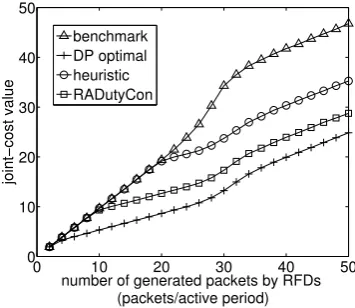
Fig. 3 shows the joint-costs of the evaluated control mech-anisms. It is shown that the proposed RADutyCon has lower joint-cost as compared to the benchmark control and the base control by the average of 31% and 19.7%, respectively, over the range of evaluated traffic. The joint-cost of RADutyCon is close to that of DP optimal control. Base on Theorem 2, the heuristic base control is the joint-cost upper bound for RADutyCon with different search ranges. The improvement of RADutyCon to the heuristic base control is achieved by searching the minimum of the cost-to-go function (20) at each time period. According toRemark 1, RADutyCon will be more beneficial when deviceni has large number of child devices,
as an exponential reduction of the computation complexity can be achieved.
0 10 20 30 40 50 0
10 20 30 40 50
number of generated packets by RFDs (packets/active period)
joint−cost value
benchmark DP optimal heuristic RADutyCon
Fig. 3. Rollout algorithm performance bound.
Fig. 4 shows the energy consumption per packet with different arrival rates. The energy consumption curves have a decrease trend along with the increase of generated packets. The change of energy consumption curve of RADutyCon between 8 packets/active period and 15 packets/active period is because the radical increase of SO, which leads to higher idle listening energy consumption. The proposed RADutyCon achieves lower energy consumption compared to benchmark control and the heuristic base control after 12 packets/active period. After 30 packets/active period, the number of trans-mitted packets is relevant stable, thus the energy consumption curves keep flat for all examined controls.
of RADutyCon begins to decrease after 20 packets per/active period. This is due to the fact that a packet can only be sent out once the existing buffered packets are cleared. With more generated packets by RFDs, the increased number of dropped packets reduces the number of buffered packets which are generated in earlier time periods. Thus, the buffer time is shortened for the packets generated in later time periods, thereby the averaged end-to-end delay is decreased. Compared with Fig. 4, it is clear that the decrease of energy consumption is at the cost of increasing end-to-end delay.
0 10 20 30 40 50
0 0.1 0.2 0.3 0.4 0.5
number of generated packets by RFDs (packets/active period)
energy consumption per packet (mJ)
benchmark DP optimal heuristic RADutyCon
Fig. 4. Energy consumption with different arrival rates.
0 10 20 30 40 50
0 5 10 15 20 25
number of generated packets by RFDs (packets/active period)
average end−to−end delay
per packet (s)
benchmark DP optimal heuristic RADutyCon
Fig. 5. End-to-end delay with different arrival rates.
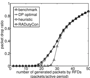
Fig. 6 shows the packet drop ratio of the evaluated control mechanisms. The packet drop ratio of RADutyCon has close performance compared with that of the heuristic base control and DP optimal control. The higher packet drop ratio than that of the benchmark control is because the reduced active periods of RADutyCon increases the number of buffered packets. Hence, the possibility of packet drop is increased due to limited maximum queue length.
VI. CONCLUSION
In this paper, we derived the optimal duty cycle control to minimise the expected joint-cost of energy consumption and end-to-end delay for 802.15.4 based WSANs. To reduce the
0 10 20 30 40 50
0 0.2 0.4 0.6 0.8 1
number of generated packets by RFDs (packets/active period)
packet drop ratio
benchmark DP optimal heuristic RADutyCon
Fig. 6. Packet drop ratio with different arrival rates.
computation complexity, RADutyCon is proposed. Simulation results shown that RADutyCon can effectively reduces the joint-cost of energy consumption and end-to-end delay under various network traffic. RADutyCon achieved lower joint-costs over the benchmark control and the heuristic base control by the average of 31% and 19.7%, respectively, over the range of evaluated traffic. The joint-cost is similar to that of DP optimal control. In addition, an exponential reduction of the computation complexity is achieved by RADutyCon.
REFERENCES
[1] M. R. Palattella, N. Accettura, M. Dohler, L. A. Grieco, and G. Boggia, ”Traffic Aware Scheduling Algorithm for Reliable Low-Power Multi- Hop IEEE 802.15.4e Networks,” inProc. IEEE International Symposium on Personal, Indoor and Mobile Radio Communications, PIMRC, September 2012.
[2] H. Byun and J. Yu, ”Adaptive Duty Cycle Control with Queue Man-agement in Wireless Sensor Networks,”IEEE Transactions on Mobile Computing, vol. 12, no. 6, pp. 1214-1224, June, 2013
[3] IEEE std. 802.15.4, Part. 15.4: Wireless Medium Access Control (MAC) and Physical Layer (PHY) Specifications for Low-Rate Wireless Personal Area Networks (LR-WPANs), IEEE Std., 2011.
[4] P. Lin, C. Qiao, and X. Wang, ”Medium Access Control With A Dynamic Duty Cycle For Sensor Networks,” in Proc. IEEE Wireless Communications and Networking Conference, WCNC, vol. 3. Atlanta, GA, USA, March 2004.
[5] S. H. Yang, H. W. Tseng, E. Wu, and G. H. Chen, ” Utilization Based Duty Cycle Tuning MAC Protocol for Wireless Sensor Networks, ” in
Proc. IEEE Global Telecommunications, GLOBECOM. Dallas, Texas, November 2005. pp. 3258 - 3262.
[6] Z. Yuqun, F. Chen-Hsiang, I. Demirkol, and W.B. Heinzelman, ”Energy-Efficient Duty Cycle Assignment for Receiver-Based Convergecast in Wireless Sensor Networks,” inProc. IEEE Global Telecommunications Conference, GLOBECOM, pp. 1-5, December 2010.
[7] X. Wang, X. Wang, G. Xing, and Y. Yao, ”Dynamic Duty Cycle Control for End-to-End Delay Guarantees in Wireless Sensor Networks,” inProc. IEEE International Workshop on Quality of Service, IWQoS, Beijing, China, June 2010.
[8] D. P. Bertsekas,Dynamic Programming and Optimal Control, 3rd Edition, Athena Scientific, 2005.
[9] T.R. Park, T.H. Kim, J.Y. Choi, S. Choi and W.H. Kwon, ”Throughput and energy consumption analysis of IEEE 802.15.4 slotted CSMA/CA,”
Electronics Letters, vol 41, no 18, 2005.
[10] H. Scarf, ”The Optimality of (s,S) Policies for the Dynamic Inventory Problem,” in Proc. of the 1st Stanford Symposium on Mathematical Methods in the Social Sciences, Stanford, CA, 1960.