Paper 16-2007

Extended Finite Element Method for Two-dimensional Crack Modeling

G. Jovicic, M. Zivkovic, N. Jovicic

University of Kragujevac,

Faculty of Mechanical Engineering,

Sestre Janjića 6, Kragujevac 34000, Serbia

e-mail: [email protected],[email protected]

Abstract

An extended finite element method (X-FEM) for two-dimensional crack modelling is described in this paper. For the crack calculation, a discontinuous function and the asymptotic crack-tip displacement fields are added to the finite element approximation using the concept Partition of Unity (PU). This enables the domain to be modelled by finite elements with no explicit meshing of the crack faces. Computational geometry issues associated with the representation of the crack and the enrichment of the finite element approximation are discussed. The presented Stress Intensity Factors (SIFs) for crack is in a good agreement with benchmark solutions. For calculation of the SIFs, we used the J-Equivalent Domain Integral (J-EDI) method.

Key words: eXtended Finite Element Method (X-FEM); Partition of Unity Method (PUM); local enrichment; elastostatics; Stress Intensity Factors (SIFs); J-Equivalen Domain Integral method (J-EDI method).

1. Introduction

The eXtended Finite Element Method, X-FEM, attempts to alleviate the computational challenges associated with mesh generation by not requiring the finite element mesh to conform to cracks, and in addition, provides use of higher-order elements or special finite elements without significant changes in the formulation. Building on prior work of Belytchko and Black [1], the basis of the method is given in [2] for two-dimensional cracks.

The essence of the X-FEM lies in sub-dividing a model problem into two distinct parts: mesh generation for the geometric domain (cracks not included), and enriching the finite element approximation by additional functions that model the flaw(s) and other geometric entities.

2. Extended Finite Element Method (X-FEM)

In this paper, the method of discontinuous enrichment is presented in general framework. We illustrate how two-dimensional formulation can be enriched for a crack model. The concept of incorporating local enrichment in the finite element partition of unity was introduced in Melenk and Babuska [3]. The essential feature is multiplication of the enrichment functions by the

nodal shape functions. The approximation for a vector-valued function _{u x}h( ) _{with the partition}

of unity enrichment has a general form [3]:

enr

1 1

( ) N ( ) M ( )

h

I I

I

N F α

α α

= =

⎛ ⎞

= _{⎜ ⎟}

⎝ ⎠

∑

∑

u x x x b (1)

where is NI, I =(1, )N are the finite element shape functions, F_α( )x , α =(1,M) are the

enrichment functions and _bα_{I is the nodal enriched degree of freedom vector associated with the}

elastic asymptotic crack-tip function that has the form of the Westergaard field for the crack tip.

The finite element shape functions form a partition of unity:

∑

note that the finite element space (F1 ≡1; Fα =0 (α ≠1)) is a subspace of the enrichment space.

We denote by N_u the set of all nodes in the domain, and N_a subset of nodes enriched by

the Heavisade function, and Nb is a subset of nodes enriched by NT (Near Tip) functions. In

particular case, for the crack, the enriched displacement approximation is written as [4, 5, 6]:

4

1

( ) ( ) ( ) ( )

u

a

b

h

I I I I

I

I

I

N H Fα α

α

∈ _∈ =

∈

⎛ ⎞

⎜ ⎟

= ⎜ + + ⎟

⎜ ⎟

⎜ ⎟

⎝ ⎠

∑

∑

u x x u x a x b

14243

14243

N

N

N

(2)

where u_I is the nodal displacement vector associated with the continuous part of the finite

element solution, a_I is the nodal enriched degree of freedom vector associated with the

Heavisade discontinuous) function.

2.1 Enrichment function

The x≡

( )

enriched functions can be used: Generalized Heavisade step function ( )H x and a set of elastic

asymptotic functions of the displacement near the crack tip (i.e. NT functions).

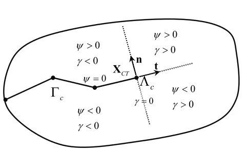
Fig. 1. Regions for enrichment near the edges of the crack.

2.1.1 Generalized Heaviside function

The interior of the crack (Γ_cis the enrichment – domain) is modelled by the generalized

Heaviside enrichment function ( )H X , where ( )H X takes the value +1 above the crack and –1

below the crack [4, 5, 6]:

*

1 if ( ) 0

( )

*

1 if ( ) 0

H _{= ⎨}⎧⎪ − ⋅ ≥

⎪ − − ⋅ <

⎩

X X n

X

X X n

(3)

where X is a sample (Gauss) point, *X (lies on the crack) is the closest point to X, and n is

the unit outward normal to crack at *X (see Fig. 2).

Fig. 2. Illustration of the values of Heaviside function above and below of the crack.

In the first published works [1,2] the above shape modelling of the discontinuity was not used. The formulation (3) began to be used due to practical numerical reasons.

2.1.2 Near-tip crack functions

Choosing the model of the crack-tip provides the representation of crack tip fields in fracture computations. Crack-tip enrichment functions are based on the Westergaard field and are used

Crack

*

X

t

n

X

C

Γ

CT X

( ) 0

H X >

( ) 0

H X < _{( ) 0 on}

C

H X = Γ

Crack Tip

in the element which contains the crack tip. The crack-tip enrichment consists of functions which incorporate the radial and angular behaviour of the two-dimensional asymptotic crack-tip displacement field.

The crack tip enriched functions ensure that the crack terminates precisely at the location of the crack-tip. Use of the linear elastic asymptotic crack-tip fields serve as suitable enrichment functions for providing the correct near-tip behaviour, and in addition, their use also leads to better accuracy on relatively coarse finite element meshes in 2D [2,4,5,6].

The crack tip enrichment functions in the isotropic elasticity have the form of the Westergaard field for the crack tip:

1 2 3 4

( ) { , , , } cos , sin , sin sin , cos sin

2 2 2 2

F = F F F F _{= ⎢}⎡ r θ r θ r θ θ r θ θ⎤_⎥

⎣ ⎦

x (4)

where is r and θ denote polar coordinates in the local system at the crack tip. It can be noted

that the second function of the set (4) is discontinuous over the crack faces [1,2]. The

discontinuity over the crack faces can be obtained using other functions, like Heaviside function (3), which have discontinuity. In [4, 5] the discontinuity behind of the tip in the CT element (element which contains the crack tip) is accomplished by the second function of the set (4). In this paper, the discontinuity in the CT element is achieved by the Heavisade function (3).

2.2 Level set representation of the crack

In this report, a crack is presented using the set of the linear segments.The crack is described by

means of the position of the tip and level set of a vector valued mapping. A signed distance

function ( )ψ x is defined over computational domainΩ as

* *

( ) ( ) min

c

sign

ψ

∈Γ

⎡ ⎤

= _⎣ ⋅ − _⎦ −

x

x n X X X X (5)

where nis the unit normal to Γc and X* is the closest point to the X, see Fig. 2. The crack is

then represented as the zero level set of the function ( )ψ X , i.e. ( ) 0

ψ X = (6)

Fig. 3. Definition of the Level Set Functions ( )ψ X andγ( )X around the crack.

The position related to the crack tip is defined through the following functions: c

Λ

CT

X n

0 0

ψ γ

> >

0

γ= ₀0

ψ γ

< >

0 0

ψ γ

< <

0 0

ψ γ

> <

0

ψ =

( ) ( _CT)

γ X = X X− ⋅t (7)

where t is the unit tangent to Γc at the crack tip Λc, and XCTis the coordinate of Λc. The

value ( ) 0γ X = corresponds to the crack tip. We define the LS functions ( )ψ X and ( )γ X in

the entire computational domain. The crack and crack tip are represented as

{

}

c ψ t γ t

Γ = X X = ∧ X ≤ (8)

In Fig. 3, the definition of ( )ψ x and ( )γ x around the crack is shown. For the crack

representations, the linear interpolation has been used. The Heavisade step function is modified using the LS function:

1 ( ) 0

( ( ))

1 ( ) 0

if H

if

γ γ

γ

− <

⎧

= ⎨_{+ >} ⎩

X X

X (9)

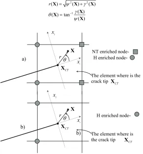
The Near tip functionsF rα( , ),θ α =1, 4, that have the form of the Westergaard field for

the crack tip [3], should also be defined using the LS functions [6] to obtain polar coordinates in the local system at the crack tip (see Fig. 4):

2 2

1

( ) ( ) ( )

( ) ( ) tan

( )

r ψ γ

γ θ

ψ

−

= +

=

X X X

X X

X

(10)

a)

b)

b)

Fig. 4. The enriched nodes of the element which contain the crack tip

a) H+NT enriched: b) H enriched.

2 x

CT

X 1

x

NT enriched node-

H enriched node-

The element where is the crack tip X_CT

X

r

_θ

CT

X 1

x H enriched node-

The element where is

the crack tip X_CT

X

r

_θ

Apart of the other authors [4, 5] we use the NT functions only ahead the crack tip ( ( , ) 0γ Xt > ); while behind the crack tip ( ( , ) 0γ Xt < ) we ensured discontinuous across the

crack ( ( , ) 0ψ Xt = ), using only the step function ( ( ))H γ X . Therefore, the Westergaard field

was used only for the derivation of the asymptotic stress field ahead the location nears the tip (see Fig. 4a) [7].

Since the NT functions are used for the cracks in the linear-elastic materials, we have considered the results in the case when the enrichment is done only by the H function (see Fig. 4b). Enrichment by H function is applied only behind the crack, hence discontinuity occurrs. This analysis is very important for further use of the X-FEM for the elastic-plastic materials.

3. Equialent domain integral method (EDI) for evaluation J-intgreal

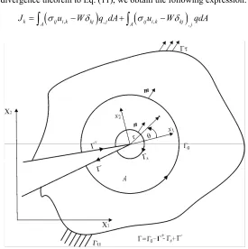
Rice [8] defined a path-independent contour J-integral for two-dimensional crack problems in linear and nonlinear elastic materials. As shown in Fig. 5, J is the line integral surrounding a two-dimensional crack tip and is defined as:

(

)

1 lim₀ 1 ,1

S S

j ij i j

J Wδ σ u n d

Γ → Γ

=

_∫

where W is the strain energy density given by:

1 1

, , , , 1, 2

2 ij ij 2 ijkl kl ij

W = σ ε = C ε ε i j k l= (12)

and nj is the outward normal vector to the contour integration, ΓS is the contour around the

crack tip (as shown in Fig. 5), σij is stress tensor, εij is strain tensor, Cijkl is constitutive tensor,

and ui is component of the displacement vector.

The contour integral (11) is not in the best suited form for finite element calculations. Therefore, the contour integral is transformed into an equivalent domain form. The equivalent domain integral method (EDI) is an alternative way to obtain the J-integral. The contour integral is replaced by an integral over a finite-size domain. The EDI approach has the advantage that the effect of variable body forces can be included easily. The standard J-contour integral given in Eq. (1 1) is rewritten, by introducing a weight function q x x

(

)

1 ,1

(Wδ _j σ_{ij i}u m qd) _j

Γ

Ψ =

_∫

where _{Γ = Γ + Γ − Γ + Γ0} + _S − _{is the contour (Fig. 5),}

j

m is a unit vector outward normal to the

corresponding contour (i.e. m_j =n_jon Γ₀ and m_j = −n_jon Γ_S), and q is a weight function

defined as q=1 inside the contour Γ and q=0 for the domain outside Γ.

0

0

,

0 0

, 0

, ,

0 0

lim lim ( )

lim ( )

lim ( ) lim ( )

S S

S S

S

S S

kj ij i k j

kj ij i k j

kj ij i k j kj ij i k j

W u m qd

W u m qd

W u m qd W u m qd

δ σ

δ σ

δ σ δ σ

+ −

+ −

Γ → Γ → Γ

Γ +Γ +Γ −Γ Γ →

Γ +Γ +Γ Γ

Γ → Γ →

Ψ = − Γ

= − Γ

= − Γ − − Γ

∫

∫

∫

∫

(14)

Applying the divergence theorem to Eq. (11), we obtain the following expression:

(

)

(

)

k _A ij i k kj j _A ij i k kj _j

J =

_∫

_∫

Fig. 5. Conversion of the contour integral into an EDI.

where A is the area enclosed by Γ. Note that the addend in the above equation must vanish for

linear-elastic materials [9, 12], so we have

(

)

k _A ij i k kj j

J =

_∫

This expression is analogous to the one proposed for a surface integral based method, to evaluate stress intensity factors.

3.1.Numerical evaluation of the J-integral

When the material of the considered structure is homogeneous, and with no body forces, the finite element implementation of Eq. (16) becomes very similar to equation of the contour

integral. The only difference is the introduction of the weight function q when Eq. (16) is used.

With the isoparametric finite element formulation, the distribution of q within the elements is

1 m

i i i

q h Q

=

=

∑

where Q_i are the values of the weight function at the nodal points, and m is the number of

nodes. The spatial derivatives of q can be obtained using the usual procedures for

isoparametric elements.

a) b)

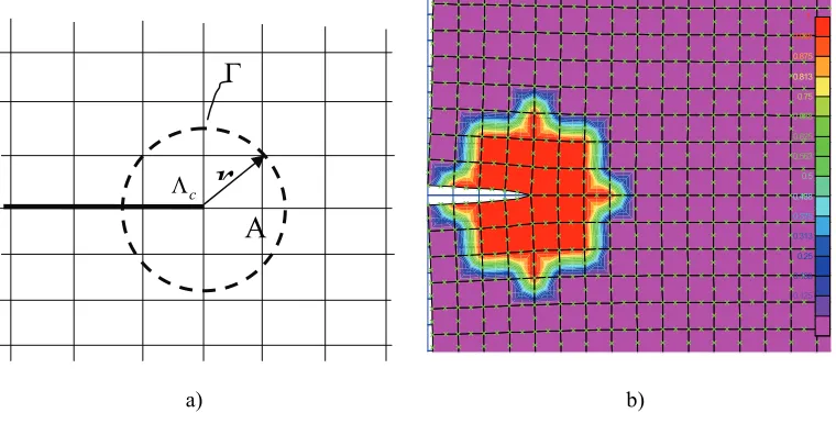
Fig. 6. The weight function q on the elements.

The equivalent domain integral in 2D can be calculated as a sum of the discretized values of Eq. (16), [9,12]:

1

det

P

i m

k ij kj p

elements p k j n

in A _p

u q X

J W w

X X

σ δ

η

=

⎡⎛ ∂ ⎞ ∂ ⎛∂ ⎞⎤

= ⎢⎜ _∂ − ⎟_∂ ⎜_∂ ⎟⎥

⎢⎝ ⎠ ⎝ ⎠⎥

⎣ ⎦

∑ ∑

The terms within

[ ]

for each point. The present formulation is adequate for a structure of homogeneous material in which no body forces are present. For the numerical evaluation of the above integral, the

domain A is a subset of the set of elements about the crack tip. Figure 6a shows a typical set of

elements for the domain A. The domain A is the set which contains all elements which have a

node within a circle of radius r_c about the crack tip. Figure 6b shows the contour plot of the

weight function q for the elements. The function q can be interpolated within the elements

using the nodal shape functions, according to Eq. (17).

4. Numerical example

To illustrate the versatility and effectiveness of the enriched approximation, the stress intensity factors are calculated using the standard FEM and X-FEM that are incorporated in the in-house software PAK [13]. In this example we determine the stress intensity factor for opening mode

of fracture (K_I) using J-EDI method. A rectangular plate with a centred crack is shown in Fig.

r

1. 0.938 0.875 0.813

0.75

0.688 0.625

0.563

0.5

0.438

0.375

0.313

0.25

0.188 0.125

0.0625 0.

A

Γ

7. The plate is subjected to uniform uniaxial tensile stress σyy at the two ends. The right half of

the model is analyzed.

Given:

7

3

1 10 5 5 3 10 0.3 1

1 25.4

1 6.89476 10

yy psi

W in

L in a in

E psi

t in

in mm

psi Pa

σ

ν = = =

= = × = =

=

= ×

Fig. 7. The centred crack in rectangular plate.

The analysis of the half model was performed using the standard FEM and X-FEM. In the standard FEM, eight-node elements and 2x2 Gauss quadrature are used. The four-node elements in the entire domain and 6x6 Gauss quadrature only in the part of the domain with enriched nodes were used in the X-FEM.

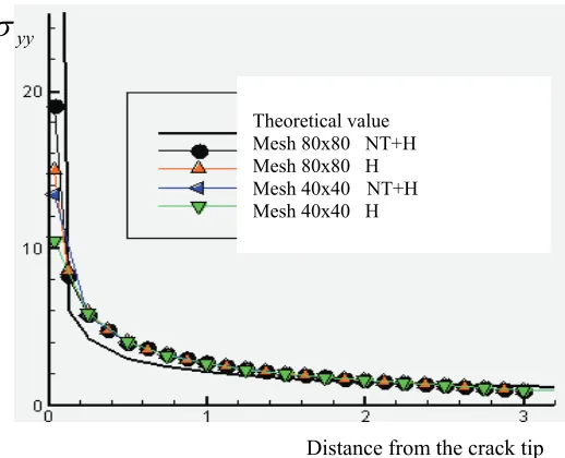
Fig. 8. The stress field σ_yyaround the crack tip. Theoretical value

Mesh 80x80 NT+H Mesh 80x80 H

Mesh 40x40 NT+H

Mesh 40x40 H

Distance from the crack tip yy

The stress field near the crack tip is asymptotic and when rc→0 (see Fig. 8), then the

stress σ → ∞_yy . The results of the stress field near the crack tip are obtained using: theoretical,

the FEM and the X-FEM, with the denisty of the mesh: 40x40 and 80x80. The example is tested in two forms using X-FEM:

a) the nodes are enriched using only Heaviside function with the meshes: 40x40; and 80x80;

b) the nodes are enriched using Heaviside function behaind crack tip and NT functions ahead

the crack tip, with the meshes: 40x40; and 80x80, (see Fig. 4).

The stress distributation near the tip of the centered crack is shwon in Fig. 9. All numerical results tend to the theoretical values. Also, it can be seen that stress in the Gauss points closest to the crack tip grows up, i.e. tends to the asymptotic value. It can be noticed that the influence of mesh density is larger than when including the NT functions. Hence, higher mesh density with H enrichment gives better results than the lower mesh density with H+NT enrichments. On the other hand, if we compare the models with the same mesh density, better results are obtained using H+NT enrichment.

The numerical results for the stress intensity factor of the first mode are compared with the theoretical results. The theoretical values are obtained using the following equation:

(

)

teor I

K =σ F a b h b πa (19)

The correction factor F a b h b

(

)

(

)

in this case it has the value F

(

)

correction factor, theoretical value of the stress intensity factor is:

7.52

teor I

K = Psi in (20)

The results for the SIF shown in the Table 1, obtained by integration of J-integral and using

J-EDI method, correspond to different integration domain rc (see Fig 6a). The radius of thhe

integration domain r_cis defined as % of the length of the crack a.

The results for the SIF are obtained using: standard FEM with 4-node discretization (FEM4), standard FEM with 8-node discretisation (FEM8), X-FEM with H enrichment (XFEM(H)) and X-FEM with H+NT enrichments (XFEM(H+NT)). In this example the same size of the elements are used in standard FEM as in the X-FEM. The difference is that the quarter of the rectangular plate with the central crack is used in the standard FEM, and half of the test model is used in the X-FEM. The results obtained using standard FEM and X-FEM are

compared with the analytical value and are shown in Table 1. Comparison is given as

(% )

c

r a KI

FEM4,40x40 KI

FEM8, 40x40 KI

XFEM(H), 40x40 KI

XFEM(H+NT), 40x40

10 11.41 7.68 7.40 7.52

15 11.61 7.65 7.52 7.55

20 11.62 7.65 6.76 6.89

25 10.41 7.40 7.51 7.56

30 11.67 7.56 7.51 7.53

35 11.69 7.60 7.50 7.51

40 11.70 7.57 7.49 7.50

Avg. vel. 11.44 7.59 7.39 7.44

N/A % 52% 0.88% 1.73% 1.06%

Table 1. Comparison of results for the SIFs obtained by FEM and X-FEM with the theoretical value

Fig. 9. Stess field arround the crack tip - model (XFEM(H), 40x40).

Fig. 10. Field of displacement normal to the crack sides, for the model with the central crack

(X-FEM model).

Stress field of the half of model, around the central crack, which is obtained using X-FEM, is shown in Fig. 9. The crack overlaps the elements edges, and there is no physical separation of the joint sides of elements. In this case, the discontinuity is modelled using the enrichment functions. It can be noticed that using the X-FEM the stress concentration is modelled at the place of the real crack tip. Displacement field around the central crack obtained by the X-FEM is shown in Fig. 10

5. Conclusion

between mesh and crack geometry, and allows arbitrary crack direction within the finite

element mesh.

In this paper we demonstrated modelling of discontinuous crack fields within an existing finite element numerical algorithm. The methodology adopted for crack modelling belongs to the class of the extended finite element method (X-FEM), which is a particular case of the partition of unity method [3]. The finite element software PAK – FM&F [13] is used in this study, and the implementation for crack modelling within isotropic media is described. The crack is described by the position of the tip and level set of a vector valued mapping. Here, the LS functions are used to determine values of NT functions. We have also modified the enrichment of the CT element.

Numerical results, obtained by these modifications, are compared with the theoretical

values, and good agreement is achieved.This study shows that the X-FEM can be incorporated

within a standard finite element package. By solving suitable test examples we showed that relatively good agreement with analytical values is obtained for the SIFs, using the standard FEM with 8-node elements and X-FEM with 4-node elements.

References

[1] T. Belytschko and T. Black, Elastic crack growth in finite elements with minimal

remeshing. International Journal for Numerical Methods in Engineering. 45(5):601-620,1999.

[2] N. Moes, J. Dolbow, and T. Belytschko, A finite element method for crack growth

without remeshing. International Journal for Numerical Methods in Engineering. 46(1):131-150,1999.

[3] J. M. Melenk and I. Babuska, The partition of unity finite element method: Basic

theory and applications, Computer Methods in Applied Mechanics and Engineering 39, 289-314, 1996.

[4] C. Daux, N. Moes, J.Dolbow, N. Sukumur, T. Belytschko, Arbitrary cracks and holes

with the extended finite element method, International Journal for Numerical Methods in Engineering 48(12),1741-1760, 2000.

[5] Sukumur N. and J.H. Prevost, Modelling quasi-static crack growth with the extended

finite element method Part I: Computer implementation, International Journal of Solids and Structures 40, 7513-7537, 2003.

[6] Jovičić G., An Extended Finite Element Method for Fracture Mechanics and Fatigue

Analysis, Ph. D. Thesis, Faculty of Mechanical Engineering, University Kragujevac, 2005.

[7] Ćulafić V.B., Itroduction in the Fracture Mechanics, Faculty of Mechanical

Engineering, University Podgorica, 1999.

[8] Rice J.R., A Path Independent Integral and Approximate Analysis of Strain

Concentration by Notches and Cracks, Journal of Applied Mechanics, 35, 379-386, 1968.

[9] Lin C-Y., Determination of the Fracture Parameters in a Stiffened Composite Panel,

Ph.D. Thesis, North Carolina State University, 2000.

[10]Kim J.-H., Paulino G.H., Mixed-mode J-integral formulation and implementation

using graded elements for fracture analysis of no homogeneous orthotropic materials, Mechanics of Materials 35 pp. 107-128; 2002.

[11]Enderlein M. Kuna M., Comparison of finite element techniques for 2D and 3D crack

[12]Jovicic G., Zivkovic M., Kojic M., Vulovic S., Numerical programs for life assessment of the steam turbine housing of the thermal power plant, From Fracture

Mechanics to Structural Integrity Assessment, Monography, Editors: S Sedmak, Z.

Radaković, 2004.

[13]Kojic M., R. Slavkovic, M. Zivkovic, N. Grujovic, G. Jovicic, S Vulovic, The software