(UDC: 530.145.6)
Adaptive modelling in atomistic-to-continuum multiscale methods
E. Marenic1,2, J. Soric2 and A. Ibrahimbegovic 1
1
Ecole Normale Supérieure de Cachan, Lab. of Mechanics and Technology, France
2Faculty of mechanical engineering and naval architecture, University of Zagreb, Croatia
Abstract
Due to the lack of computational power to perform a fully atomistic simulation of practical, engineering systems, a number of concurrent multiscale methods is developed to limit atomic model to a small cluster of atoms near the hot spot. In this paper the overview of salient features of the main multiscale families is given. The special attention is drawn towards the role of model adaptivity, that is, which part of the problem domain to model by the atomic scale (the hot spot) and which by coarse scale model, as well as where to place the interface of the two models to control the accuracy. Taking Quasicontinuum method as a reference, review of the evolution of the Bridging domain/Arlequin method is given, which parallels the development of a posteriori modeling error estimation.
Keywords: molecular mechanics, atomistic-to-continuum coupling, quasicontinuum, bridging domain, Arlequin, Cauchy-Born rule, RVE, goal error estimates, goals algorithm
1 Introduction
The emphasis of scientific research in material science has shifted from micro- and meso-scale to the study of the behavior of materials at the atomic scale of matter. The first trends of this kind go back to the 1980s. when the scientists and engineers began to include atomistic descriptions into models of materials failure and plasticity [Buehler 2008]. This research is related to the terms nano-technology and nano-mechanics. At nano-scale, the effects of single atoms, individual molecule, or nano-structural features may dominate the material behavior, especially at failure [Buehler 2008]. The classical continuum mechanics, that has been the basis for most theoretical and computational tools in engineering [Ibrahimbegovic 2009], is not suitable for nano-scale applications. Thus, different kind of computational modeling, in particular atomistic and/or molecular simulation, has become increasingly important in the development of such new technologies [Cleland 2003, Rapaport 2004, Phillips 2004].
instrumentation can observe and characterize forces of the order of hundreds of pN, with displacements of the order of nanometers [Buehler 2008]. Atomistic simulation has been used in the research topics like: the atomic-scale effect in fracture and wear, dislocation dynamics in nano-indentation, nano-composites, carbon nano tubes, nano electro mechanical system components, semiconductors and biomechanics [Buehler ,7].
The main challenge is that atomistic models typically contain extremely large number of particles, even though the actual physical dimension may be quite small. For example, even a crystal with dimensions below a few micrometers sidelength has several tens of billions of atoms. Predicting the behavior of such large particle systems under explicit consideration of the trajectory of each particle is only possible by numerical simulation, and must typically involve the usage of the supercomputers [Buehler 2008]. Even though nanoscale systems and processes are becoming more viable for engineering applications, our ability to model their performance remains limited, since the fully atomistic simulations remain out of reach for engineering systems of practical interest.
Multiscale (MS) modeling methods have recently emerged as the tool of choice to link the mechanical behavior of materials from the smallest scale of atoms to the largest scale of structures [Wing et al 2006]. MS methods are often classified as either hierarchical or concurrent. Hierarchical methods are the most widely used, for their computationally efficiently. In these methods, the response of a representative volume element (RVE) at the fine scale is first computed, and from this a stress-strain law is extracted. Thus, the computations are performed on each scale separately and the scale coupling is often done by transferring the problem parameters leading to the classical problem of homogenization (e.g. see early work [Sanchez-Palencia 1980]). For severely nonlinear problems, hierarchical models become more problematical, particularly if the fine scale response is path dependent. It should be noted that when failure occurs, in many circumstances hierarchical models are invalid and cannot be used [Fish 2009].
Concurrent methods, on the other hand, are those in which the fine scale model (e.g. atomistic, treated with molecular mechanics) is embedded in the coarse scale model (usually continuum model treated with FEM) and is directly coupled to it. In the study of fracture, for example, fine scale models can be inserted in hot spots where stresses become large and where there is the biggest risk of failure. These hot spots can be identified on the fly or by a previous run. Molecular mechanics (MM) and/or quantum mechanics (QM) models are required for phenomena such as bond breaking, but the relevant configuration is far too large to permit a completely atomistic description. In order to make such problems computationally tractable, the molecular model must be limited to small clusters of atoms in the vicinity of a domain of interest where such high resolution models are necessary and a continuum method should be used for the rest of the domain [Fish 2009]. Here we primarily focus on the concurrent, static (equilibrium), atomistic-to-continuum MS modeling, strongly coupling atomistic and continuum scales.
coupling, it can be used as a reference for adaptive strategy. More precisely, the question we thus address pertains to which part of the domain should be modeled by the fine (atomic) scale and which by coarse scale model in a particular problem, and where to place the interface of the two models to control the accuracy for any solution stage?
The paper is organized as follows. Following this introduction, the paper starts with the short overview of atomic models in Section 2 and finishes with the motivation for the MS methodology and a short list of leading MS methods. Then the standard QC and BD/Arlequin methods are described in Sections 3 and 4, respectively. Following the general description of the two methods the comparison is summarized in 5. Numerical examples of model adaptivity are presented in Section 6 in order to illustrate these ideas, and provide quantitative comparison between different adaptive modelling strategies. The concluding remarks are stated in Section 7.
2 Atomistic (particle) model
2.1 Atomistic interaction modeling
The first choice that should be made for any kind of material modeling is the energy function describing the system of interest. Once the energy of the atomic interaction is defined, the essential of material behavior is determined. The main goal of this section is to give a general introduction to atomistic i.e. non-continuum material modeling, to introduce the essential ideas and review the literature. It is worth to mention that the reason for introducing the atomistic modeling is two-folded. First, the atomistic modeling is used as a testing ground for energetics of the system, by using the simplest generic form of the interaction model. Second, the potential function (U) driving the molecular system can take an extremely complicated form, when the goal is to represent the quantitative predictions for specific material. In this case, an accurate representation of the atomic interactions has to be material specific. The nature of these interactions is due to complicated quantum effects taking place at the subatomic level that are responsible for chemical properties such as valence and bond energy [Wingat al 2006, Ercolessi1997, Griebel et al 2007]. However, quantum mechanics based description of atomic interaction is not discussed herein, emphasis is rather on the empirical interaction models that can be derived as the result of such computations. Alternatively, the function U in classical interatomic potential that can be obtained from experimental observations and should accurately account for the quantum effects in the average sense. However, many different expressions can be fit to closely reproduce the energy predicted from quantum mechanics methods (semi-empirical), while retaining computational efficiency [Buehler 2008, Allen and Tildesley 1987]. Needless to say, there is no single approach that is suitable for all materials and for all different phenomena of material behavior that we need to describe. The choice of the interatomic potential depends very strongly on both the particular application and the material.
The general structure of the potential energy function for a system of N atoms is
practical reasons is when the sum in (1) is truncated after second term resulting with the pair-wise potential.
2.2 Pair-wise potentials
The total energy of the system in pair potentials is given by summing the energy of all atomic bonds 1 ( ( )) over all N particles in the system.
∑ ∑ ( ) ∑ ∑ ( ) (2)
Note the factor 1/2 accounts for the double counting of atomic bonds. One of the most well known interatomic potentials is the Lennard-Jones (LJ), or yet called 6-12 potential. The potential energy function for the LJ potential is expressed as
(
) ((
)
(
) ), (3)
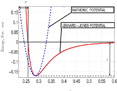
where and are constants chosen to fit material properties (no relation to continuum stress and strain, see Fig. 1) and is the distance between two atoms i and j. The term is meant to model the repulsion between atoms as they approach each other, and is motivated by the Pauli principle in chemistry. The Pauli principle implies that as the electron clouds of the atoms begin to overlap, the system energy increases dramatically because two interacting electrons cannot occupy the same quantum state. The term adds cohesion to the system, and is meant to mimic van der Waals type forces. The van der Waals interactions are fairly weak in comparison to the repulsion term, hence the lower order exponential is assigned to the term. LJ 6-12 is an example of potential limited to the simulations where a general class of effects is studied, instead of specific physical properties, and a physically reasonable yet simple potential energy function is desired [Harold and Park 2004].
Since the LJ potential is highly nonlinear function of the atom pair distance , it is sometimes useful to use its linearized form in terms of so-called harmonic potential
( ) ( ) , (4)
where is the initial (equilibrium) atomic pair distance, and is the bond stiffness. The harmonic potential can describe the atomic system behavior for small atomistic separation (refer Fig. 1). Hence, this potential is usually chosen as the first and simplest description of the atomic interaction, in particular in development of the MS methods where the emphasis is on the coupling and not on the accurate and realistic description of different material mechanisms.
Fig. 1. Lennard-Jones and Harmonic potential (dashed line). Note that the Harmonic potential is a suitable approximation when the particles are around the equilibrium position.
2.3 Embedded atom method (EAM) potentials and multi-body potentials
This kind of interaction models are widely used to model metals [Daw and Baskes 1983, Doyama and Kogure 1999]. A local density dependent contribution is added to the pair potential energy function (2) by embedding energy term F
∑ ( ) ∑ ( ) (5)
The embedding energy ( ) is related to the environment of the atom i, and is the local electron density. The main advantage of this kind of potential is the ability to describe surfaces or cracks since they incorporate the variation of bond strength with coordination (density).
A number of different approaches to realistic description of behavior of solids based on the first-principles or quantum mechanical calculations have been developed in recent decades. These models account for the environmental dependence of the bond strength with the force between any two particles depending upon the position of several neighbouring particles. Besides EAM, the other examples of this kind of potentials are Finnis and Sinclair potential describing metallic bonds, and the Brenner potential used for hydrocarbon bonds [Griebel et al 2007].
2.4 Solution strategy and motivation for MS methods
We focus in this work upon the mechanics behavior only, in the context of quasi-static loading applications. The equilibrium configuration of solids corresponds to a state of minimum energy. Similar to the FEM, that the positions of all nodes are determined by minimizing the energy in the solid. Thus, for a system of N atoms, the equilibrium configuration is determined by minimizing
∑ ̅ . (6)
of FEM, see e.g. [Liu et al 2004, Liu et al 2005, Liu et al 2008, Wang et al 2006, Wackerfuß 2009].
The task of minimizing (6) quickly becomes intractable for large number of particles (atoms). This, together with the assumption that the calculation of specific quantities of the solution can be accurately approximated by replacing the particle model by a coarser model (i.e. continuum model), is the basis for multiscale (MS) modeling. Extensive work has been done in the development of atomistic-to-continuum MS modelling approaches, starting with early works by [Mullins and Dokainish 1982] and [Kohlhoff et al. 1990]. Mullins simulated 2D cracks in -iron with the atomic scale models, and due to the restrictions of the computational power the question was how to connect the atomic model and surrounding continuum. Kohlhoff et al. proposed a new method for combined FE and atomistic analysis of crystal defects, called FEAt. Both papers dealt with the problem of proper treatment of the transition between the lattice and continuum.
A number of MS methods developed recently from theoretical standpoint of view appear very different. However, as shown in [Miller and Tadmor 2009], at the implementation level all these methods are in fact very similar. The performance of a number of most frequently used methods is compared in a linear framework on a common benchmark test. The ways in which various multiscale methods differ are the formulation (energy or force based model), the coupling boundary conditions, the existence of the handshake region (overlapped or non-overlapped domain de-composition), and the choice of the continuum model. The list containing: quasicontinuum (QC) method (in Section 3), bridging domain (BD) method (in Section 4), coupling of length scales (CLS), bridging scale (BS) method [Harold and Park 2004, Karpov et al 2006, Qian et al 2004], coupled atomistics and discrete dislocations (CADD), Atomistic-to-continuum coupling (AtC) [Fish et al 2007, Badia et al 2007, Badia et al 2008], etc. is also not exhaustive but the unified framework, available computer code, and a quantitative comparison between the methods offer a good overview. Note that there is also a very recent effort of coupling non-local to local continuum [Han and Lubineau 2012] in the Arlequin framework (see Section 4). An alternative to discrete modeling of atomic/particle systems is the use of non-local continuum mechanics models (NLCM) [Lubineau et al 2012]. NLCM reduces the computational costs but has the ability to capture non-local interactions. However since the simulation using NLCM is also costly due to assembly operation of the discretized model where each interaction point interacts with multiple neighbours, and the fact that this reduces the sparsity of the matrices, similar principle as in BD and QC method of coupling discrete, non-local particle model with local continuum is used. The key challenge is then again the gluing of non-local continuum model with the local one.
The standard approach in these models is to a priori identify the atomistic and continuum regions and tie them together with some appropriate boundary conditions. In addition to the disadvantage of introducing artificial numerical interfaces into the problem a further drawback of many of these models is their inability to adapt to changes in loading and an evolving state of deformation. Take for example the problem of nanoindentation. As the loading progresses and dislocations are emitted under the indenter the computational model must be able to adapt and change in accordance with these new circumstances.
3. Quasicontinuum method
The Quasicontinuum (QC) method is originally proposed in late 90‘s by Tadmor, Ortiz and Phillips [Tadmor et al 2012]. Since then it has seen a great deal of development and application by a number of researchers. The QC method has been used to study a variety of fundamental aspects of deformation in crystalline solids, including fracture [Miller et al 1998, Miller et al 1998, Hai and Tadmor 2003] 2 , grain boundary slip and deformation [Shenoy et al 1999]. The nano-indentation [Shenoy et al 2000] and similar applications are examples where neither atomistic simulation nor continuum mechanics alone were appropriate, whereas the QC was able to effectively combine the advantages of both models. The main goal of the QC method is the provide a seamless link of the atomistic and continuum scales. This goal is achieved by the three main building blocks [Eidel et al 2010, Miller and Tadmor 2002]:
1. Reduction of degrees of freedom (DOF) by coarse-graining of fully atomistic resolution via kinematic constraints. The fully atomistic description is retained only in the regions of interest.
2. An approximation of the energy in the coarse grained region via numerical quadrature. The main idea is to avoid the need to calculate the energy of all the atoms, but retain only a few so-called rep-atoms.
3. Ability of the fully re?ned, atomistic region to evolve with deformation, where adaptivity is directed by suitable re?nement indicator.
3.1 DOF reduction or coarse graining
If the deformation changes gradually on the atomistic scale, it is not necessary to explicitly track the displacement of every atom in the region. Instead it is suffcient to consider some selected atoms, often called representative atoms or rep-atoms. This process is in essence the upscaling via coarse graining. Only rep-atoms have independent DOF while all other atoms are forced to follow the interpolated motion of the rep-atoms. The QC incorporates such a scheme by means of the interpolation functions of the FE method, and thus the FE triangulation has to be performed with rep-atoms as FE mesh nodes. This way continuum assumption is implicitly introduced in QC method. Thus, if the potential is given as a function of displacement u (similarly as in (6))
( ) ( ) ∑ ̅
, (7)
Where ̅ is the external force on the atom i and is an atomistic internal energy
∑ (
), (8)
the kinematic constraint described above is performed by replacing , with
∑ (
). (9)
In the above equation the displacement approximation is given via standard FE interpolation
∑ ( )
, (10)
3.2 Efficient energy calculation via Cauchy-Born rule
Described kinematic constraint on most of the atoms in the body will achieve the goal of reducing the number of degrees of freedom in the problem. However, for the purpose of energy minimization the energy of all the atoms (not just rep-atoms) has to be computed. The way to avoid visiting every atom is the Cauchy-Born (CB) rule [Ericksen 1984, Ericksen 2008, Zanzotto 1996]. The CB rule postulates that when a simple, mono-atomic crystal is subjected to small displacement on its boundary then all the atoms will follow this displacement. In QC this rule is implemented in that every atom in a region subject to a uniform deformation gradient will be energetically equivalent. Thus, energy within an element can be estimated by computing the energy of one, single atom in the deformed state. The estimation is performed simply by multiplying the single atom energy by the number of atoms in the speci?c element. The strain energy density (SED) of the element can be expressed as:
( ) ( ), (11)
where is s the energy of the unit cell when its lattice vectors are distorted according to deformation gradient F, and is the volume of unit cell. The sum in eq. (9) is reduced to number of FEs ( )
∑ ( )
, (12)
where the element volume and unit cell volume are related as , and is the number of atoms contained in element e. Using the CB rule, the QC can be thought of as a purely continuum formulation (local QC), but with a constitutive law that is based on atomistic model rather than on an assumed phenomenological form [Miller and Tadmor 2002]. Within QC framework, the calculation of CB energy is done separately in a subroutine. For a given deformation gradient F the lattice vectors in a unit cell are deformed according to given F and the SED is obtained according to eq. (11).
3.3 Non-local QC and local/non-local coupling
In settings where the deformation is varying slowly and the FE size is adequate with respect to the variations of the deformation, the local QC is sufficiently accurate and very effective. In the non-local regions, which can be eventually refined to fully atomistic resolution, the energy in (9) can be calculated by explicitly computing only the energy of the rep-atoms by numerical quadrature
∑ ( )
(13)
where is the weight function for rep-atom i and is high for atoms in regions of low rep-atom density and low for high density. Thus, is the number of the atoms represented by the i -th rep-atom wi-th -the limiting case of for fully atomistic case and consistency requirement
∑
. (14)
The main advantage of the non-local QC is that when it is refined down to the atomic scale, it reduces exactly to lattice statics.
∑ ( )
∑ ( ), (15)
where the weights n i are determined from the Voronoi tessellation i.e. by means of the cells around each rep-atom. The cell of atom i contains atoms, and of these atoms reside in FE
e adjacent to rep-atom i. The weighted energy contribution of rep-atom i is then found by applying the CB rule within each element adjacent to i such that
∑ ( ), ∑ , (16)
where is the cell volume for single atom, and is the number of FE adjacent to atom i.
3.4 Local/non-local criterion
The criterion to trigger the non-local treatment is based on the significant variation of deformation gradient 3 . Precisely, we say that the state of deformation near a representative atom is nearly homogeneous if the deformation gradients that it senses from the different surrounding elements are nearly equal. The non-locality criterion is then:
| | , (17)
where is the k-th eigenvalue of the right stretch tensor for element a, k = 1 . . . 3 and indices a and ( ) refers to the neighboring elements of rep-atom. The rep-atom will be made local if this inequality is satisfied, and non-local otherwise, depending on the empirical constant .
3.5 Adaptivity
Without a priori knowledge of where the deformation field will require fine-scale resolution, it is necessary that the method should have a built-in, automatic way to adapt the finite element mesh through the addition or removal of rep-atoms. This is a feature that is in QC inherent from the FE literature, where considerable attention has been given to adaptive meshing techniques for many years. Typically in FE techniques, a scalar measure is defined to quantify the error introduced into the solution by the current density of nodes (or rep-atoms in the QC). Elements in which this error estimator is higher than some prescribed tolerance are targeted for adaptation, while at the same time the error estimator can be used to remove unnecessary nodes from the model.
4 Bridging domain and Arlequin-based coupling
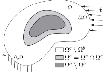
The Bridging domain (BD) method is in essence a partially overlapping domain decomposition scheme used for atomistic-to-continuum coupling developed by Belytschko and Xiao in 2003 [Belytschko and Xiao 2003] for the static, and [Xiao and Belytschko 2004] for dynamical problems. The compatibility in the overlapping domain is enforced by Lagrange multipliers. The evolution of the aforementioned method (see also [Zhang et al 2007, Anciaux et al 2008, Belytschko et al 2010]) has much in common with recent works in the finite element (FE) community on the coupling of nonconforming meshes in the overlapping subdomain. This approach is known as Arlequin method developed by Ben Dhia [Dhia and Rateau 2005, Dhia et al 2008, Guidault and Belytschko 2007]. The same Arlequin approach is lately also applied for atomistic-to-continuum coupling like in [Bauman et al 2008, Prudhomme et al 2008, Bauman et al 2009, Guidault and Belytschko 2009, Prudhomme et al 2009, Chamoin et al 2010, Dhia et al 2010]. More precisely, the domain with models coupling of is divided in three subdomains as shown in Fig. 2. The atomistic domain is discretized with molecular dynamics or rather molecular mechanics (MM), whereas the continuum mechanics domain discretization is carried out by FEs. The atomistic and continuum domains overlap in the domain . This overlapping domain is also called bridging, handshake or coupling domain. The role of the continuum
Fig. 2. Scheme of the coupled model and the nSM technique.
model is to replace the molecular model with a coarser, and thus computationally cheaper, model in away from the region of interest (e.g. lattice defect). Initially emphasis of the research was to make the coupling of the two different models as seamless as possible. No special attention was devoted to the question how to adaptively refine the model around the region of interest and where to position the handshake zone i.e. how far from the region of interest.
4.1 Construction of surrogate model
The role of the surrogate model is to propagate only the large-scale information. The choice of this model depends on the nature of the material but it should be selected as the most ‘compatible‘ model with the atomistic or particle model in the sense of homogenization [62]. Thus, the material parameters of the surrogate continuum constitutive model should be calibrated accordingly. To that end, there are two approaches that appear in the BD/Arlequin literature.
2004, Zhang et al 2007]. The Cauchy-Born rule is described in detail in section 3.2. The second approach pertains to computing the equivalent continuum model parameters through homogenization. Simple illustration for 1D case is given in [Bauman et al 2007] for the case of linear elastic continuum. More systematic approach to calibrating the continuum model parameters exploits the virtual experiments on the representative volume element (RVE) as suggested in [Prudhomme et al 2009]. The continuum model is based on plane stress linear elasticity and the constitutive relation is defined by Hooke‘s law. A RVE is considered to be a piece of material (atomistic lattice in this case) whose dimension is increased in iteratively until the consistent homogenized medium is obtained where the material parameters do not vary with further size increase. The lattice samples are larger than the effective RVEs in order to avoid boundary effects. The choice of the continuum model is, naturally, problem dependent (see [Bauman et al 2009] for nonlinear hyperelastic material model suitable for polymeric materials).
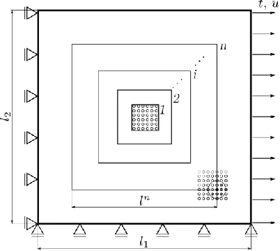
An example of the (virtual) experiment for the uniaxial tension case is described in sub-sequently. Let the lattice sample size be with constraints on the left and bottom atom layers, and imposed force (to obtain traction t) or displacement u on every right-most atom Fig. 3. Without loss of generality we take the pair-wise interaction, where the internal energy
Fig. 3. Scheme of the lattice sample and increasing square shaped RVEs (1, 2, . . . , i, . . . , n) increasing until material parameters convergence. Due to simplicity, only RVE 1 is shown as a
lattice structure.
of the RVE is calculated as in (2) with . The strain energy density is calculated by dividing the atomic energy by the initial volume of the RVE ( )
. (18)
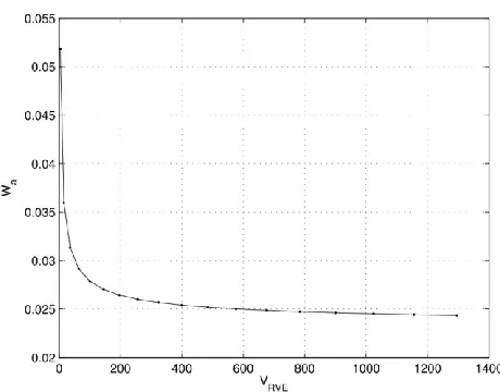
Fig. 4. Atomistic strain energy density ( ) convergence with increasing size of RVE.
that the energy densities obtained from the continuum and atomistic models are identical, so that 5 , where W is continuum strain energy density. Such value of W is further used to
calculate the continuum part of energy (as indicated in equations (19) and (20)). This kind of approach obviates the need for the CB hypothesis to be fulfilled, which is used for composite lattices e.g. in 1D setting [Chamoin et al 2010].
4.2 Governing equations and coupling
Total potential energy of the system may be written as
( ) ( ) ( ), (19)
where u i d are displacement vectors in the continuum and atomistic domains, respectively. Furthermore, is the work of external forces, while and are weighted continuum and atomistic energies, defined as
( ) ∫ ( ) ( ) ( ) ∑ . (20)
In the bridging domain the two models overlap, and the weighting functions and in (20) partition the energy. The weighting function serves to blend the behavior from the continuum model ( ) and the atomistic model ( ) and to avoid the double counting of the energy in the bridging domain. Furthermore, the use of an overlapping subdomain obviates the need for the FE nodes of the continuum model to correspond to the atomic positions. The weighting functions and define a partition of unity of the energy in the bridging domain as follows:
( )
( )
( ) ( )
(21)
Fig. 5. Energy weighting function distribution in the bridging zone.
overburden that illustration. Already in early contributions by [Belytschko and Xiao 2003, Zhang et al 2007] the discrete coupling of the atomistic and continuum models was achieved by forcing displacement compatibility in the bridging domain as ( ) . There, the Lagrange multiplier (LM) method was used to convert the problem of constrained minimization into finding the minimum of the larger, unconstrained problem. Hence, LMs, denoted with , are used to enforce the compatibility between the discrete atomistic displacement (discretely for each atom within the coupling zone) and the continuum displacement field. This results with the following Lagrangian
∑ ∫ ( ) ( ) ( ) , (22)
where C is the constraint in terms of the energy. In numerical implementation, displacement field in and LM fields in are approximated by using, respectively, the shape functions
( ) and ( ) as
( ) ∑ ( ) ( ) ∑ ( ) ̂ , (23)
with and ̂ as the corresponding nodal values. Two limit cases regarding the LM field approximation are: i) the strict (or so called non-interpolated or atomic/particle) coupling with the LMs defined with atoms in the bridging zone and where i.e. ( ) ) the interpolated (or continuum) coupling where the -nodes coincide with FE nodes and the LM shape functions correspond to the FE shape functions . The distribution of the -nodes for the two cases is illustrated in Fig. 6 for 1D case.
Fig. 6. Scheme of the distribution of the LM nodes for strict and interpolated coupling.
∫ ( ) , (24)
∫ ( ) ( ) ( ) , (25)
where l has the unit of a length, and corresponds to a characteristic dimension of the coupling zone. Apart from the advances in the coupling itself which is mostly related to the development of the Arlequin method advocated in initial work by Ben Dhia [Dhia and Rateau 2005] and its further application to the atomistic-to-continuum coupling, this method is acquiring the ability to accommodate the model and decrease the error in chosen quantity of interest. That is, the adaptivity described above for the QC method was included in the BD/Arlequin. This evolution parallels recent development in goal oriented error estimate theory as discussed in forthcoming section.
4.3 Adaptivity and error estimate
In computer simulations of physical models there are two major sources of error. Approximation error due to the discretization of mathematical models, and modeling error related to the simplification or in general to the natural imperfections in abstract models of actual physical phenomena. The focus is here on the estimation and control of modeling error. This subject has been introduced in recent years and was initially devoted to estimating global modeling error e.g. [Ainsworth and Oden 1997]. Since then, extensions to error estimates in specific quantities of interest (estimate upper and lower bounds of error in linear functionals) have been proposed [Oden and Vemaganti 2000, Oden and Prudhomme 2002, Prudhomme et al 2003]. As an example Oden and Vemaganti [Oden and Vemaganti 2000] proposed an extension of a posteriori modeling error estimation for heterogeneous materials to the quantities of interest so-called goal-oriented error estimates. Many candidates for local quantities of interest are de facto quantities that one actually measures when assessing mechanical response e.g. average stresses on material interfaces, displacement, etc. Mathematically, a quantity of interest is any feature of the ?ne-scale solution that can be characterized as a continuous linear functional on the space of functions to which the ?ne-scale solution belongs. Analogously as in [Oden and Vemaganti 2000], where the error estimates are related to the error between ?ne-scale and regularized (homogenized) model, goal-oriented error estimation is extended to the case of discrete models (lattice) in [Oden et al 2005]. That is, this approach is used to estimate the modeling error between the atomic structure (lattice) and the surrogate, continuum model (i.e. FE discretization of the continuum model).
The idea behind the goal oriented adaptive modeling (as shown in the mentioned references) is to start from coarse, regularized model and to adaptively proceed towards fine model. Hence, the model is adopted to deliver local quantity of interest to within preset accuracy. The general process of adapting the surrogate model in order to decrease the modeling error in specific quantities of interest is referred to as the Goals Algorithms.
as atomic displacement, and the second one ( ) as average force on atom. The associated modeling errors are ( ) ( ), where . This convergence study shows decrease of the mentioned modeling errors with the increase of the . This analysis was a first step6 , and a basis for the development of the adaptive strategy.
Finally, the Goals algorithm is extended to the Arlequin based coupled atomic-to-continuum modeling [Prudhomme et al 2009, Dhia et al 2010]. The adaptive procedure that controls the error is obtained by generating a sequence of surrogate problems so that the modeling error satisfies:
( ) ( ) , (26)
where is predefined tolerance. Reduction of the modeling error at each iteration is done by locally enriching the surrogate model, i.e. by locally switching on the atomic model in the subregions where the continuum model is not accurate enough 7. Modeling error is defined globally over the whole domain but can be decomposed into local contributions (subdomains). Naturally, the elements of the finite element mesh used to discretize the continuum model are chosen as subdomains or cells. Now, some user-defined parameter (subdomain tolerance similar as ) is chosen to decide when can the subdomain be switched from the continuum model to the particle model.
5 MS methods comparison
In the foregoing, we have given an overview of the mainstream MS methods in terms of QC method and BD/Arlequin based coupling. The latter currently attracts the greatest attention with many BD/Arlequin recent developments, but it still has not been fully completed as the simpler, but well known QC method. Therefore, we try to present in this section the comparison of these two methods, hoping to be able to draw lessons on further improvements to the present practise. This comparison is carried out regarding: 1. coupling algorithm, 2. continuum modeling, 3. applicability, and finally 4. adaptivity strategy.
5.1 Coupling algorithm
The coupling algorithm of these two methods are drastically different. QC method seeks to provide a gradual transition, where the mesh composed of repatoms as nodes is gradually refined starting from the local towards the non-local description. This gradual transition is numerically more convenient regarding its capability to reduce the ill-conditioning. However, it also has a few drawbacks. First of all, an enormous refinement has to be performed in going from the FE continuum representation to the atomistic lattice size. Furthermore, the FE nodes and the atoms have to coincide. Contrary to that, BD/A method couples the two models only in the zone of partial overlap. Neither gradual transition nor coincidence between the nodes and elements are needed. However, atomistic and continuum DOFs are completely separated and additional unknowns in terms of Lagrange multipliers that enforce the coupling need to be accounted for. In addition, in order to avoid double counting the blending of the energy in overlapping domain is done by weighting functions, which also have to be chosen appropriately.
5.2 Continuum modeling
structures 8 . On the other hand, due to use of classical coupling of atomic and continuum domains, The BD/A method offers another approach to defining the surrogate (homogenized) continuum model. Namely, fitting the material parameters by virtual experiments on RVE, the atomistic part is reduced to the corresponding continuum. Thus, there is no need for CB hypothesis to be satisfied.
5.3 Applicability
During development period of the QC method, it served both as a key vehicle for understanding of the nature of atomistic-continuum coupling, and as a practical tool for investigating problems requiring coupled atomistic-continuum solution procedure. Nowadays, there is a unified web site qcmethod.org as the original source of information, with publications and the most important download section. Under the download section the QC code is available written in Fortran90 by the Tadmor and Miller. On the other hand, BD/A method was not used that much as a practical tool (apart some application to carbon nano tubes by Xiao and Belytschko), it was more used for the theoretical testing of different aspects of coupling and MS modeling in general. However the method is from the very beginning extended to dynamics, dealing with spurious wave reflections in the transition from the atomic to continuum domain. There is no unified web site as for QC method, but there are examples like libmultiscale.gforge.inria.fr.
5.4 Adaptivity strategy
Original QC method is in essence an adaptive FE approach, and adaptivity is intrinsically in the formulation in QC method. BD/A method was initially assumed as approach to couple two different models. However, the described evolution associated with the goal oriented error estimate theory, with the strong mathematical foundations, improved the method so that it is equal if not better compared to the QC method in the sense of model adaptivity. In particular, the choice where to place the fine and where to remain with coarse scale model, and how to provide the appropriate evolution of that region is still the most important question. More precisely, the BD/A method adaptivity is driven by the goals algorithm, controlling the model refinement with respect to the any chosen quantity of interest. In QC method non-locality criterion is based on a significant variation in the deformation gradient (no other criteria). In very recent contributions the model adaptivity is being combined with optimal control theory and shape optimization allowing size and shape of the zone of interest to be automatically determined (or controlled in the sense of the error in the quantity of interest).
6 Numerical examples with model adaptivity
We present further some numerical examples that can clearly demonstrate the model adaptivity for the BD/A based coupled model. The accuracy of chosen quantities of interest (QOI) is used as the measure of the model adaptivity performance. Contrary to QC method, there are many candidates for local QOIs, and the best choice certainly depends on the problem on hands. In the examples the follow, the quantities are selected for the sake of overview: Q1 -displacement of the rightmost node, Q2 - L2 norm of displacement error in overlapping zone, Q3 - mean strain in the overlapping zone, Q4 - L2 norm of strain error in overlapping zone, Q5 - stress difference between neighbouring bonds. Next to QOIs, some other parameters of the model ought to be selected selected, and properly adapted. These parameters are divided in two groups. The first one pertains to the shape i.e. size of the overlap along with the size of the FEs for continuum domain. The second group concerns the size of the ?ne scale (particle) domain
i.e. to issue where to place the overlap.
6.1 Adapting model topology - FE and overlap size
In this example, we demonstrate the influence of the model topology on the accuracy of QOIs Q1 . . . Q4. The accuracy improvement is performed in the simple, chainlike (1D) problem as in Fig. 7 (see Section 4 and [Marenic et al 2012]). Two parameters are taken into consideration for the
topology adaptation: the size of the FE ( ), and the size of the overlapping zone ( ). In extension, local (only ) and nonlocal ( and , see Fig. 7) types of interaction are selected in the atomistic domain and taken as the third parameter.
Parameter 1: the size of the FE
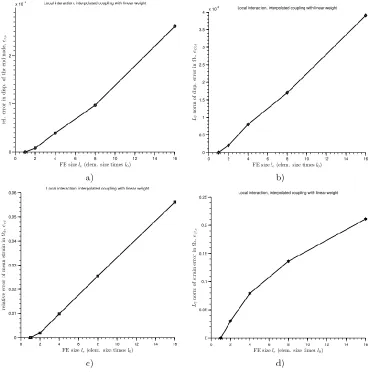
For the local, non-interpolated case of the model problem the solution of the full molecular and coupled model show no error in the mentioned QOIs with the variation of the parameter . On the other hand, for the case of interpolated coupling within the local interaction in , the error in the QOIs exists and it is shown in the Fig. 8 with respect the variation of the parameter . In the analysis of the influence of parameter upon the QOIs, the other parameter (the size of the overlapping zone) is kept constant ( ). On the
Fig. 8. Local interaction in with FE size as a parameter. Quantities of interest Q1,
Q2, Q3 and Q4 are shown on plots denoted as a), b), c) and d), respectively.
( ) , (27)
where and is the displacement of the rightmost node and the exact value for the displacement, respectively. Note that in the examples presented herein, the exact values refer to the fully molecular (or particle) solution.
On the Fig. 8 b) relative L 2 norm of the displacement error in the overlapping zone is given as
√∑ ( )
√∑ ( )
, (28)
where and are atom displacement solution ( ) for the coupled model and the exact solution, respectively. The relative error in Q3, the mean strain in the overlapping zone, is given on Fig. 8 c) as
̅ ̅ ̅ ̅ , (29)
where ̅ and ̅ are the mean strain in overlapping zone and exact mean strain, respectively. Likewise, on the Fig. 8 d) relative norm of the strain error in the overlapping zone is given as
√∑ ( )
√∑ ( )
, (30)
where and are strain solution ( ) for the coupled model and the exact solution, respectively.
Similarly, the same analysis is performed with the non-local interaction in atomistic domain. The results are shown in the Fig. 9 indicating the same tendency as for local interaction with the bigger error. Note that for all the plots in Figs. 8 and Fig. 9 the errors in QOIs drops down to zero as the size of the FE decreases to lattice constant being . This result is rather logical, since decreasing the FE size for the interpolated coupling case we approach the non-interpolated case (see Fig. 6) where no error occurs, as already mentioned above.
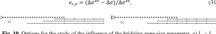
Parameter 2: the size of the bridging zone
6.2 Adapting the position of the overlap
In this section the parameter for adapting the coupled model is the position of the overlap zone with respect to the strain gradient caused by distributed load or by hypothetical defect. Actually, the position of the overlap is directly related to the fine scale model size, that is to the question pertaining to the size of the fine-scale model.
Fig. 9. Nonlocal interaction in with FE size as a parameter. Quantities of interest Q1, Q2, Q3 and Q4 are shown on plots a), b), c) and d), respectively.
6.3Model with distributed load
mentioned three cases is plotted on Fig. 13. Not quite surprising, the presented results show better accuracy in terms of selected QOIs as the particle size is increased (i.e. as the distributed load is further from the overlap). Furthermore, QOI Q5 representing stress difference between neighbouring bonds is taken as the control variable to adapt the ?ne scale size. The relative error in Q5 is defined as
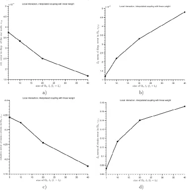
( ) , (31)
Fig. 10. Options for the study of the influence of the bridging zone size parameter. a) = and b) = cst.
where and is the exact stress difference and the one obtained from coupled model, respectively (see Fig. 14 a)). Stress difference is obtained as , i.e. the difference of stress (piece-wise constant) in the neighbouring bonds. Results of the relative error in stress difference of the leftmost atom in the overlap versus the position of overlap is presented in Fig. 14 b). The results show that the error in terms of stress QOI decreases with the increase of the size of fine scale model. Clearly, when the strain gradient, caused by the distributed load, is in fine scale model completely the error in stress QOI does not exist. This QOI provides a very good local refinement criterion. We note in passing that such a QOI, apart from being a good refinement criteria, can be related to the often mentioned ghost forces problem. Thus, choosing this QOI Goals algorithm can be used to iteratively adapt coupled model to increase the coupling quality i.e. ghost forces. This is more important for complex interatomic potential with non-local interaction, which is the subject of forthcoming research.
6.4 Model with defect
Next, a model with the defect is analyzed. This defect is modeled as the sudden stiffness change (see Fig. 15 a)) which occurs inside the particle domain. Problem is similar as the distributed load but with a more severe strain gradient. According to the adaptive scheme in Fig. 15 b) the fine-scale model size is increased. Not surprisingly, adapting the model in a way that the defect (severe strain gradient) is included in fine scale model, reduces the error in QOIs as can be seen in Fig. 16.
7 Conclusions and perspectives
In the consideration where nano-scale effects are important, the reference solution can be obtained by using the full atomic model relying upon interatomic potentials to provide the results of interest. However, due to the complexity of engineering problems and the corresponding scales that appear in realistic problems, explicit modeling of all with only the atomic degrees of freedom will very likely never be feasible. Thus, one must reduce the size of the problem by multiscale strategies (MS) that selectively removes most of the degrees of freedom by homogenized continuum formulation in order to make the problem solution tractable.
removing of degrees of freedom i.e. model adaptivity is neglected. The QC method is based on adaptive approach, thus being an exception and the reference for comparison in this review survey. The evolution of the BD/A method from atomistic-to-continum coupling to adaptive MS method is presented, as well as the literature regarding error estimation theory which parallels the development.
The general idea of model adaptivity is demonstrated on few numerical examples. The presented examples deal with the simplest 1D case, and they should not be used to quantify computational efficiency or the limits of adaptive criteria (tolerances). The idea was,
Fig. 11. Local interaction in with size of ( ) as a parameter. Quantities of interest Q1, Q2, Q3 and Q4 are shown on subplots a), b), c) and d), respectively.
Further perspectives of the BD/A method development is related to the implementation of the complex multi-body potential which enables more realistic description of the discrete model. In many such case, the complex potential is even more computationally demanding as elaborated in the Section 2, which additionally justifies using the MS strategy. The use of this kind of potentials enables modeling of inelastic behavior and localized failure at the nano-scale. Equally, those potentials are able to describe the behavior of ‘living‘ material in life science. Both of this issues are presently very important in the technical and biomechanics research domain (e.g. see Kojic et al. [Kojic et al 2008, Kojic 2008]).
Fig. 12. Three cases of the position of the bridging zone with respect to the distributed load 1) distributed load (q) not in overlap, 2) q partially in overlap and 3) q on all atoms, completely
covering the overlap.
Fig. 13. Local interaction in with position of distributed load as a parameter (for L2 and H1 coupling, see eq. 24). Quantities of interest Q1 and Q2 are shown on plots a) and b),
Fig. 14. a) stress plot for the model that for the model that needs refinement. The stress difference for the coupled model and referential, particle model are shown, and b) relative error
in stress difference of the leftmost atom in the overlap versus the position of overlap.
Fig. 15. Modeling of defect by the sudden spring stiffness drop located on the left end a), and characteristic cases regarding the overlap position (d 0 ) with respect to the defect radius (R def
Извод
Адаптивно моделирање у мултискалним методама од атомске до
континуум скале
E. Marenic1,2, J. Soric2 and A. Ibrahimbegovic 1
1
Ecole Normale Supérieure de Cachan, Lab. of Mechanics and Technology, France
2Faculty of mechanical engineering and naval architecture, University of Zagreb, Croatia
Резиме
Због недостатка компјутерске снаге да се уради потпуна атомистичка симулација практичних, ижењерских система, један број садашњих мултискалних метода је развијен да ограничи атомистички модел на мали кластер атома у близини значајне тачке. У овом раду се даје преглед најбитнијих карактеристика основних мултискалних фамилија. Посебна пажња је посвећена улози адаптивности метода, тј. који део домена проблема да се моделира на атомској скали (значајна зона), а која са моделом на грубој скали, као и питање где поставити границу између два модела да би се контролисала тачност. Узимајући Квазиконтинуум методу као референтну, дат је преглед развоја методе повезивања домена, односно Арлеквин методе (Bridging domain/Arlequin method), који је паралелан са развојем накнадне (a posteriori) процене грешке моделирања.
Кључне речи: молекуларна механика, повезивање атом-континуум, квазиконтинуум, повезивање домена, Арлеквин , Коши-Борн правило, РВЕ (референтна еквивалентна запремина), циљна процена грешке, циљни алгоритам.
References
M. J. Buehler. Atomistic Modeling of Materials Failure. Springer US, 2008. 1, 2, 3
A. N. Cleland. Foundations of Nanomechanics From Solid-State Theory to Device Applications.Springer, 2003. 1
D. C. Rapaport. The Art of Molecular Dynmics Simulations. Cambridge University Press,2004. 1
R. Phillips. Crystals, Defects and Microstructures Modeling Across Scales. Cambrifge Uni-veristy press, 2004. 1
M. J. Buehler. Atomistic and continuum modeling of mechanical properties of collagen: Elas-ticity, fracture, and self-assembly. J. Mater. Res., 21:1947–1961, 2006. 2
M. J. Buehler. Nanomechanics of collagen fibrils under varying cross-link densities: Atomisticand continuum studies. Journal of the Mechanical Behavior of Biomedical Materials, 1(1):59– 67, 2008. 2
H. S. P. Wing Kam Liu, Eduard G. Karpov. Nano Mechanics and Materials Theory, MultiscaleMethods and Applications. John Wiley & Sons, Ltd, 2006. 2, 3
E. Sanchez-Palencia. Non-homogeneous media and vibration theory. Springer, 1980. 2
W. A. Curtin and R. E. Miller. Atomistic/continuum coupling in computational materialsscience. Modelling Simul. Mater. Sci. Eng., 11:33–68, 2003. 2
W. K. L. Harold S. Park. An introduction and tutorial on multiple-scale analysis in solids.Computer Methods in Applied Mechanics and Engineering, 193:1733–1772, 2004. 2, 4, 6
W. K. Liu, E. G. Karpov, S. Zhang, and H. S. Park. An introduction to computational nanomechanics and materials. Computer Methods in Applied Mechanics and Engineering,193(17-20):1529 – 1578, 2004. 2
R. Rudd and J. Broughton. Concurrent coupling of length scales in solid state systems. Physica status solidi (b), 217:251–291, 2000. 2
R. E. Miller and E. B. Tadmor. A unified framework and performance benchmark of four-teen multiscale atomistic/continuum coupling methods. Modeling and Simulation in Materials Science and Engineering, 17:053001, 2009. 2, 6
J. Q. Broughton, F. F. Abraham, N. Bernstein, and E. Kaxiras. Concurrent coupling of length scales: Methodology and application. Phys. Rev. B, 60(4):2391–2403, Jul 1999. 2
D. Srivastava and S. N. Atluri. Computational nanotechnology: A current perspective. CMES,3:531–538, 2002. 2
F. Ercolessi. A molecular dynamics primer, June 1997. 3
M. Griebel, S. Knapek, and G. Zumbusch. Numerical Simulation in Molecular Dynamics. Springer, Berlin, Heidelberg, 2007. 3, 5
M. P. Allen and D. J. Tildesley. Computer simulation of liquids. Oxford Univeristy press, 1987.3
R. Sunyk. On Aspects of Mixed Continuum-Atomistic Material Modelling. PhD thesis, Fach-bereich Maschinenbau und Verfahrenstechnik der Technischen Universit at Kaiserslautern,2004. 4, 16
M. S. Daw and M. I. Baskes. Embedded-atom method: Derivation and application to impuri-ties, surfaces, and other defects in metals. Physical Review, 29:6443–6453, 1983. 5
M. Doyama and Y. Kogure. Embedded atom potentials in fcc and bcc metals. Computational Materials Science, 14(1-4):80 – 83, 1999. 5
B. Liu, Y. Huang, H. Jiang, S. Qu, and K. C. Hwang. The atomic-scale finite element method. Computer Methods in Applied Mechanics and Engineering, 193(17-20):1849 – 1864, 2004. 5
B. Liu, H. Jiang, Y. Huang, S. Qu, M.-F. Yu, and K. C. Hwang. Atomic-scale finite element method in multiscale computation with applications to carbon nanotubes. Phys. Rev. B,72(3):035435, Jul 2005. 5
B. Liu, Z. Zhang, and Y. Chen. Atomistic statics approaches - molecular mechanics, finite element method and continuum. Journal of computational and theoretical nanoscience, :1891–1913, 2008. 5
Y. Wang, C. Zhang, E. Zhou, C. Sun, J. Hinkley, T. S. Gates, and J. Su. Atomistic finite elements applicable to solid polymers. Computational Materials Science, 36(3):292 – 302,2006. 5
J. Wackerfuß. Molecular mechanics in the context of the finite element method. International Journal for Numerical Methods in Engineering, 77:969–997, 2009. 5
M. Mullins and M. Dokainish. Simulation of the (001) plane crack in alpha-iron employing a new boundary scheme. Philosophical Magazine A, 46:771–787, 1982. 6
S. Kohlhoff, P. Gumbsch, and H. F. Fischmeister. Crack propagation in b.c.c. crystals studied with a combined finite-element and atomistic model. Philosophical Magazine A, 64:4:851 —878, 1991. 6
D. Qian, G. J. Wagner, and W. K. Liu. A multiscale projection method for the analysis of carbon nanotubes. Computer Methods in Applied Mechanics and Engineering, 193(17-20):1603– 1632, 2004. 6
J. Fish, M. A. Nuggehally, M. S. Shephard, C. R. Picu, S. Badia, M. L. Parks, and M. Gun-zburger. Concurrent AtC coupling based on a blend of the continuum stress and the atomistic force. Computer Methods in Applied Mechanics and Engineering, 196(45-48):4548 – 4560, 2007.6
S. Badia, P. Bochev, R. Lehoucq, M. Parks, J. Fish, M. A. Nuggehally, and M. Gunzburger. A force-based blending model foratomistic-to-continuum coupling. International Journal for Multiscale Computational Engineering, 5(5):387–406, 2007. 6
S. Badia, M. Parks, P. Bochev, M. Gunzburger, and R. Lehoucq. On atomistic-to-continuum coupling by blending. Multiscale modeling and simulation, 7-1:381–406, 2008. 6
F. Han and G. Lubineau. Coupling of nonlocal and local continuum models by the arlequin approach. International Journal for Numerical Methods in Engineering, 89(6):671–685, 2012. 6
G. Lubineau, Y. Azdoud, F. Han, C. Rey, and A. Askari. A morphing strategy to couple non- local to local continuum mechanics. Journal of the Mechanics and Physics of Solids, 60(6):1088– 1102, 2012. 6
E. B. Tadmor, M. Ortiz, and R. Phillips. Quasicontinuum analysis of defects in solids. Philo-sophical Magazine A, 73:1529–1563, 1996. 6
R. Miller, E. B. Tadmor, R. Phillips, and M. Ortiz. Quasicontinuum simulation of fracture at the atomic scale. Modeling and Simulation in Materials Science and Engineering, 6:607–638, 1998. 7
R. Miller, M. Ortiz, R. Phillips, V. Shenoy, and E. B. Tadmor. Quasicontinuum models of fracture and plasticity. Engineering Fracture Mechanics, 61(3-4):427 – 444, 1998. 7 S. Hai and E. B. Tadmor. Deformation twinning at aluminum crack tips. Acta
Materialia,51(1):117 – 131, 2003. 7
V. B. Shenoy, R. Miller, E. b. Tadmor, D. Rodney, R. Phillips, and M. Ortiz. An adaptive finite element approach to atomic-scale mechanics–the quasicontinuum method. Journal of the Mechanics and Physics of Solids, 47(3):611 – 642, 1999. 7, 10
V. B. Shenoy, R. Phillips, and E. B. Tadmor. Nucleation of dislocations beneath a plane strain indenter. Journal of the Mechanics and Physics of Solids, 48(4):649 – 673, 2000. 7
B. Eidel, A. Hartmaier, and P. Gumbsch. Atomistic simulation methods and their applica-tion on fracture. In R. Pippan, P. Gumbsch, F. Pfeiffer, F. G. Rammerstorfer, J. Salen¸con, B. Schrefler, and P. Serafini, editors, Multiscale Modelling of Plasticity and Fracture by Means
of Dislocation Mechanics, volume 522 of CISM Courses and Lectures, pages 1–57. Springer Vienna, 2010. 7
R. E. Miller and E. B. Tadmor. The quasicontinuum method: Overview, applications and current directions. Journal of Computer-Aided Materials Design, 9:203–239, 2002. 7, 8, 9 J. L. Ericksen. The cauchy and born hypotheses for crystals. Phase transformation and material
instabilities in solids - from book ‘Mechanics and Mathematics of Crystals: Selected Papers of
J. L. Ericksen‘ by Millard F. Beatty and Michael A. Hayes, page 61–77, 1984. 8
J. Ericksen. On the cauchy–born rule. Mathematics and Mechanics of Solids, 13:199–220, 2008.8
G. Zanzotto. The cauchy-born hypothesis, nonlinear elasticity and mechanical twining in crystals. Acta Crystallographica, A52:839–849, 1996. 8
S. P. Xiao and T. Belytschko. A bridging domain method for coupling continua with molecular dynamics. Computer Methods in Applied Mechanics and Engineering, 193(17-20):1645 – 1669, 2004. 10, 11
S. Zhang, R. Khare, Q. Lu, and T. Belytschko. A bridging domain and strain computation method for coupled atomistic-continuum modelling of solids. International Journal for Multi-scale Computational Engineering, 70:913–933, 2007. 10, 11, 13
G. Anciaux, O. Coulaud, J. Roman, and G. Zerah. Ghost force reduction and spectral analysis of the 1d bridging method. Research Report RR-6582, INRIA, 2008. 10
T. Belytschko, R. Gracie, and M. Xu. A continuum-to-atomistic bridging domain method for composite lattices. International Journal for Numerical Methods in Engineering, 81:1635– 1658,2010. 10
H. B. Dhia and G. Rateau. The Arlequin method as a flexible engineering design tool. Inter- national Journal for Numerical Methods in Engineering, 62:1442–1462, 2005. 10, 14 H. B. Dhia, N. Elkhodja, and F.-X. Roux. Multimodeling of multi-alterated structures in the
Arlequin framework. solution with a domain-decomposition solver. European Journal of Computational Mechanics, 17:969 – 980, 2008. 10
P.-A. Guidault and T. Belytschko. On the l2 and the h1 couplings for an overlapping domain decomposition method using lagrange multipliers. Int. J. Numer. Meth. Engng., 70:322– 350,2007. 10
P. T. Bauman, H. B. Dhia, N. Elkhodja, J. T. Oden, and S. Prudhomme. On the application of the arlequin method to the coupling of particle and continuum models. Computational Mechanics, 42:511–530, 2008. 10, 11, 13
S. Prudhomme, H. B. Dhia, P. Bauman, N. Elkhodja, and J. Oden. Computational analysis of modeling error for the coupling of particle and continuum models by the Arlequin method. Computer Methods in Applied Mechanics and Engineering, 197(41-42):3399 – 3409, 2008. Recent Advances in Computational Study of Nanostructures. 10, 14
P. T. Bauman, J. T. Oden, and S. Prudhomme. Adaptive multiscale modeling of polymeric materials with arlequin coupling and goals algorithms. Computer Methods in Applied Mechanics and Engineering, 198:799 – 818, 2009. 10, 11
P. Guidault and T. Belytschko. Bridging domain methods for coupled atomistic-continuum models with l2 or h 1 couplings. International Journal for Numerical Methods in Engineering,77-11:1566–1592, 2009. 10, 13
S. Prudhomme, L. Chamoin, H. B. Dhia, and P. T. Bauman. An adaptive strategy for the control of modeling error in two-dimensional atomic-to-continuum coupling simulations. Computer Methods in Applied Mechanics and Engineering, 198(21-26):1887 – 1901, 2009. Advances in Simulation-Based Engineering Sciences - Honoring J. Tinsley Oden. 10, 11, 13, 15
L. Chamoin, S. Prudhomme, H. Ben Dhia, and T. Oden. Ghost forces and spurious effects in atomic-to-continuum coupling methods by the arlequin approach. International Journal for Numerical Methods in Engineering, 83:1081–1113, 2010. 10, 11, 12, 13
H. B. Dhia, L. Chamoin, J. T. Oden, and S. Prudhomme. A new adaptive modeling strategy based on optimal control for atomic-to-continuum coupling simulations. Computer Methods in Applied Mechanics and Engineering, In Press, Corrected Proof:–, 2010. 10, 14, 15
H. Qiao, Q. Yang, W. Chen, and C. Zhang. Implementation of the Arlequin method into ABAQUS: Basic formulations and applications. Advances in Engineering Software, 42(4):197– 207, 2011. 13
J. Oden and K. S. Vemaganti. Estimation of local modeling error and goal-oriented adaptive modeling of heterogeneous materials: I. error estimates and adaptive algorithms. Journal of Computational Physics, 164(1):22 – 47, 2000. 14
J. Oden and S. Prudhomme. Estimation of modeling error in computational mechanics. Journal of Computational Physics, 182(2):496 – 515, 2002. 14
S. Prudhomme, J. T. Oden, T. Westermann, J. Bass, and M. E. Botkin. Practical methods for a posteriori error estimation in engineering applications. International Journal for Numerical Methods in Engineering, 56(8):1193–1224, 2003. 14
J. Oden, S. Prudhomme, and P. Bauman. On the extension of goal-oriented error estimation and hierarchical modeling to discrete lattice models. Computer Methods in Applied Mechanics and Engineering, 194(34–35):3668 – 3688, 2005. 14
R. Sunyk and P. Steinmann. On higher gradients in continuum-atomistic modelling. International Journal of Solids and Structures, 40(24):6877 – 6896, 2003. 16
E. Marenic, J. Soric, and Z. Tonkovic. Nano-submodelling technique based on overlapping domain decomposition method. Transactions of FAMENA, 36:1–12, 2012. 17
M. Kojic, N. Filipovic, B. Stojanovic, and N. Kojic. Comuter Modelling in Bioengineering – Theory, Examples and Software. Wiley, 2008. 22
M. Kojic. On the application of discrete particle methods and their coupling to the continuum based methods within a multiscale scheme. Monograph of Academy for Nonlinear Sciences, 2:357–356, 2008. 22

![Fig. 7 (see Section 4 and [Marenic et al 2012]). Two parameters are taken into consideration for the](https://thumb-us.123doks.com/thumbv2/123dok_us/8371068.1675210/17.499.78.455.510.582/fig-section-marenic-et-al-parameters-taken-consideration.webp)