point of failure) and positive (improved balancing flexibility) properties. The objective of this paper is we discuss the performance requirements of the DNS, and argue that the robustness and performance of the DNS could be improved and also discuss the impact of TTL on response time in DNS
I. INTRODUCTION
The Domain Name System (DNS) is one of the components most critical to Internet functionality. Nearly all Internet applications rely on the DNS for name-to-address translation. The ubiquity of the DNS necessitates both the accuracy and availability of responses.At the most basic level, Domain Name System, or DNS as it is commonly known, is an Internet service that maps domain names into IP addresses and is an essential component of any network. There are two types of DNS servers: authoritative and non-authoritative.
1. Authoritative DNS Authoritative DNS is the authoritative source for all DNS requests made for a designated domain.
2. Non-Authoritative DNS Also referred to as a Local DNS (LDNS) or a caching DNS server -- is often located near the DNS client, caching DNS answers received from Authoritative DNS servers, speeding future resolution requests. Local DNS servers are usually provided by ISPs or an enterprise’s IT department.
Load balancing both authoritative and non-authoritative DNS servers requires handling DNS queries coming from a variety of sources. The minor difference between the two is that the non-authoritative DNS servers need to make outbound connections to other authoritative DNS servers, while authoritative DNS servers require zone transfers. In a small to medium-size load environment, DNS servers may be both authoritative and authoritative. In a large environment, DNS servers may be dedicated to serve as either authoritative or non-authoritative.
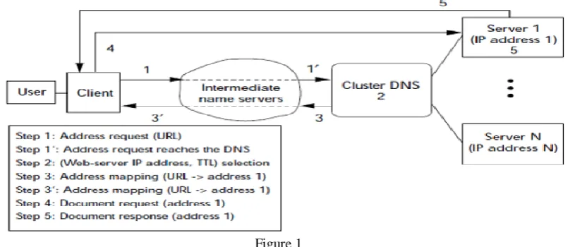
II. DNS ARCHITECTURE
Figure 1
Problems exist even at the network-level of address caching because most intermediate name servers are configured such that they reject very low TTL values [1][2][3].
III. DNS ALGORITHM
There are three common lookup methods used in open-source DNS servers. (We do not address the data structures used in commercial servers as the source code is not available to us.)
The first, and most common, is a balanced binary search tree using a comparison function that implements the DNS’s ordering on names. This is used in BIND, NSD and many less-popular servers.
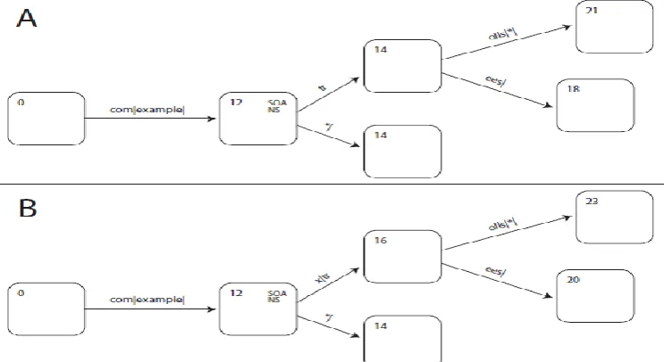
The second is to store all RRSets in a hash table , indexed by the query name and type. This allows for very fast lookups but requires some special handling for failed lookups, such as explicitly searching for the enclosing zone or wildcard. The third is to offload the data lookup to a general-purpose database, using a standard interface such as SQL or Berkeley DB. Using a database back-end allows administrators to integrate their other network management tools with their DNS zones without needing to export zone files. For example the DNS namespace, and a trie holding the same names. In order to preserve the same ordering on DNS names as required for DNSSEC, we must first reorder the labels, so www.example.com is entered in the trie as com|example|www|, where | separates labels and is ordered before all other characters. Also, any upper-case ASCII characters are converted to lower case. With these
Figure 2: The same names arranged in a radix trie
The zone head is stored at last soa, and the cut point for a delegated zone is at last ns. If the lookup succeeded, the RRSets for the queried name are at node. If the lookup failed before the key was used, we report a name error (NXDomain); if it failed and all the key was used, we report a “no data” error (NoError).
For example, in the first zone fragment in Figure 7.4 a lookup of the name trial.example.com should be answered from the RRSets of *.example.com. In the second, although the tries have the same shape, a lookup for trial.x.example.com should fail. Algorithm 2 shows how
this can be implemented in the radix trie.
Figure 3: Examples of the DNS wildcard algorithm
3.1 Updates
the IP address of a server he controls. He then creates files on the server he controls with names matching those on the target server. These files could containmalicious content, such as a computer worm or a computer virus. A user whose computer has referenced the poisoned DNS server would be tricked into accepting content coming from a non-authentic server and unknowingly download malicious content.
4.1 DNS anticipation and improvement
Many cache poisoning attacks can be prevented on DNS servers by being less trusting of the information passed to them by other DNS servers, and ignoring any DNS records passed back which are not directly relevant to the query. For example, versions of BIND 9.5.0-P1[3] and above perform these checks.[4] As stated above, source port randomization for DNS requests, combined with the use of cryptographically-secure random numbers for selecting both the source port and the 16-bit cryptographic nonce, can greatly reduce the probability of successful DNS race attacks.
BIND (Berkeley Internet Name Domain) [7] is the most commonly used Domain Name System (DNS) server on the Internet. The earliest BIND servers did very little to address security. In order to avoid a same transaction ID repeating at the same time in the network, the server used an “Increment by One” method. Each new query was issued with the previous transactionID+1. Guessing the transaction ID in such a case is a fairly easy job. This weakness was patched and the new BIND versions issue a random transaction ID to every new query. In the new version (BIND 9), the transaction ID is a randomly generated number, or more precisely, the transaction ID is a pseudo random generated number. The algorithm that generates the IDs in each of the BIND versions is open to the public and can be easily obtained and studied. As shown in [8], in many of the BIND 9 versions, the algorithm is weak and the next random number can be derived from the previous one
However routers, firewalls, proxies, and other gateway devices that perform network address translation (NAT), or more specifically, port address translation (PAT), often rewrite source ports in order to track connection state. When modifying source ports, PAT devices typically remove source port randomness implemented by nameservers and stub resolvers. Secure DNS (DNSSEC) uses cryptographic electronic signatures signed with a trusted public key certificate to determine the authenticity of data. DNSSEC can counter cache poisoning attacks, but as of 2008 was not yet widely deployed. In 2010 DNSSEC was implemented in the Internet root zone servers.[5]Although, some security experts claim with DNSSEC itself, without application-level cryptography, the attacker still can provide fake data.[6] This kind of attack may also be mitigated at the transport layer or application layer by performing end-to-end validation once a connection is established. A common example of this is the use ofTransport Layer Security and digital signatures. For example, by using HTTPS (the secure version of HTTP), users may check whether the server's digital certificate is valid and belongs to a website's expected owner. Similarly, the secure shell remote login program checks digital certificates at endpoints (if known) before proceeding with the session. For applications that download updates automatically, the application can embed a copy of the signing certificate locally and validate the signature stored in the software update against the embedded certificate.
V. TTL ALGORITHM
request is again forwarded to authorized DNS. Setting this value to very small or zero does not work because of existence of non cooperative intermediate name servers and client level caching. Also, it increases network traffic and DNS itself can become bottleneck. Several DNS based approaches are discussed in and . DNS based algorithms can be classified on the basis of the scheduling algorithms used for server selection and TTL values. Constant TTL algorithms: These are classified on the basis of the system state information used by DNS for server selection. The system state information can include both client and server state information, like load, location etc.[1]
1. System stateless algorithms : Most simple and first used algorithm of this type is round robin (DNS-RR). It was used by NCSA (National Center for Supercomputing Applications) to handle large traffic volume using multiple servers. In this approach, primary DNS returns IP addresses of servers in the round robin fashion.
It suffers from uneven load distribution and server overloading, since large number of client from same domain (using same proxy/gateway) are assigned same server. Also, whole document tree must be replicated on every server or network file system should be used.
2. Server state based algorithms : A simple feedback mechanism from servers about their loads is very effective in avoiding server overloading and not giving IP address of unavailable servers. The scheduling policy might be to select the least loaded server any time. This approach solves overloading problem to some extent yet control over requests is not good because of caching of IP addresses. Some implementations try to solve this problem by reducing TTL value to zero but it is not generally applicable and puts more load on DNS.[9][10]
(a) Client state based algorithms : In this approach, two types of information about clients, the typical load arriving to system from each connected domain (from same proxy/gateway) and the geographical
proximity can be used by DNS for scheduling.
Requests arriving from domains having higher request rate per TTL value can be assigned to more capable server. Proximity information can be used to select nearest server to minimize network traffic. One mode of Cisco Distributed Director [11] takes client location (approximated from client's IP address) and client-server link latency into account to select the client-server by acting as primary DNS. This approach also suffers form same problem experienced by Server state based algorithms.
(b) Server and Client state based algorithms : Cisco Distributed Director takes server availability information along with client proximity information into account while making server selection decision. These algorithms can also use various other state estimates for server selection. Such algorithms give the best results.
(c) Dynamic TTL algorithms : These algorithms also change TTL values while mapping host name to address. These are of two types :
a. Variable TTL algorithms : As server load increases these algorithms try to increase DNS control over request distribution by decreasing TTL values.
b. Adaptive TTL algorithms : These algorithms take into account the domain request rate (number of requests from a domain in TTL time period) and server capacities, for assigning TTL values. So a large TTL value can be assigned for a more capable server and less TTL value for those mappings that have high
domain request rate.
These are most robust and effective in load balancing even in presence of skewed loads and non-cooperative name servers, but these don't take geographical information into account.[12]
VI. EXPERIMENTAL RESULT
6.1 Impact of TTL on Response-time 1. Static Back-end
Figure 4: Flood static – Total page load time. This plot shows the total page load time, DNS lookup + HTTP request, observed by running the flood tool against the shared web server address. Note the relatively low
deviation for TTL 0.
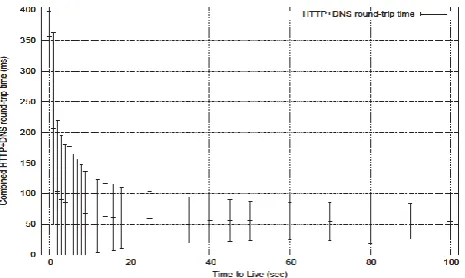
Figure 5: Flood static – DNS lookup times. This is a probability density plot for the round-trip times observed in DNS lookups for a varying TTL. We clearly see the two peaks at x = 20 and x = 300
Figure 6: Flood static – DNS lookup times (scaled). This figure is a scaled version of the previous plot. Scaling is individual for both peaks, to better observe their properties. Note the characteristic dip around x = 280 for
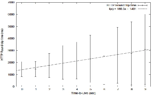
2. Dynamic Back-end
When exchanging the static BIND back-end with a highly flexible and dynamic PowerDNS setup, an administrator is given a very powerful tool that can aid in manageability and performance. When analysing the network dump files gathered from the client, we observed a rise in both round-trip time and deviation as the TTL was increased. The plot in figure 7 is derived from the network dumps and shows this relationship. What we observe is a steady and almost perfectly linear increase in HTTP response time corresponding to the input TTL value. For TTL 0, we observe a relatively low response time with comparably low standard deviation. Since we use a zero TTL, all DNS lookups are directed to the authoritative source, which returns a random entry from the set of six addresses, i.e. a one in six chance for returning any given address. Since we get a new address for each HTTP request, the scheduling granularity is very fine; all servers participate equally in answering the heavy requests. Incidentally, the measurements for TTL 1 are almost exactly the same as for TTL 0. A cause for this could be that the request rate from the client is less than one per second, which would result in a zero cache hit-rate. This is not the case, however: The flood configuration is set up to generate. Consider figure 8, where we see a time series plot of the load for each server for TTL 0 (a) and 20 (b). The measurements were gathered at a resolution of one second, but were smoothed out using a simple moving average with a window of ten seconds. For a zero TTL, it is apparent that no server reaches 100% CPU utilisation. The load is rather unstable, but is generally kept well below 50%. On a side note, the plot for TTL 0 clearly shows the four different flood sessions, starting around 0, 110, 220 and 360 seconds, respectively. When we increase the TTL to 20, the outcome is markedly different probability. . A service operator would be interested in keeping the probability of overload as low as possible, and could analyse data flows to determine a suitable TTL to achieve this goal. Another interesting point to look at is the HTTP response times as plotted in figure 9, using the cumulative frequency distribution. Using this approach, we can observe that for TTL 0, most requests – nearly 90% – are within the range of 0 to 1,000 ms per request. Conversely for TTL 9, around 60% of requests are within a range of 0 to 2,000 ms/req. Similarly, a TTL of 9 seconds also results in approximately 90% of requests lie within the 0 to 6,000 ms/req range. Results of this kind is what forms the basis of service level agreements, where providers guarantee some levels of service for customers; e.g. a level can define minimum delays with a given probability
(a) Server load with TTL 0
b) Server load with TTL 20
Figure 8: Web server utilisation with varying TTL. The figures show the observed load on all six web servers during the testing, for TTLs 0 and 20.
Figure .9: Flood dynamic – Cumulative HTTP response time. This graph shows the cumulative frequency distribution of response times for HTTP queries. A higher TTL leads to a higher degree of delayed responses,
because of higher possibility of over-utilisation.
VII. CONCLUSION
Throughout this paper, we have examined the use of the Domain Name System as a mechanism for load balancing. Insight into available literature on the topic has shown that DNS lookups are an often neglected, yet substantial part of total page response time – not only because of network traversal delay, but because of the recursive nature of queries. The use of caching offers a partial remedy to this challenge of mitigating the frequency of time-intensive authoritative lookups, but introduces problems of its own. Caching time for a given resource record is governed by the time-to-live parameter set at the authoritative nameserver for that record. A TTL of a few seconds suggests that auth lookups are frequent, and the cache hit-rate is low. A TTL of hours to days would mean a considerably higher cache hit-rate, but forfeits the ability of the authoritative nameserver to influence the information within the much longer period until TTL expiry. Further, we have investigated aspects of popular DNS implementations and their practice of answering of requests, both for caching and authoritative modes. Based on a varying set of input parameters, our goal has been to determine the degree of uncertainty in meeting QoS demands, especially that of round-trip times.
REFERENCES
[1] Cardellini, Colajanni, and Philip S. Yu, ―Dynamic Load balancing on web-server systems‖, published in
IEEE internet Computing, vol. 3, no. 3, pp 28-39, 1999.
[2] Cardellini, Colajanni, and Philip S. Yu, ―Dynamic Load Balancing in geographically Distributed Heterogeneous Web Server‖, published in the proceedings of IEEE 18th International Conference on Distributed Computing Systems, at Amsterdam, The Netherlands, pp, 295-302, May 1998.
[3] "BIND Security Matrix". ISC Bind. Retrieved 11 May 2011. [4] "ISC Bind Security". ISC Bind. Retrieved 11 May 2011.
[5] "Root DNSSEC". ICANN/Verisign. p. 1. Retrieved 5 January 2012. [6] "DNS forgery". Retrieved 6 January 2011.
[7] D. B. Terry, M. Painter, D. W. Riggle, and S. Zhou, “The Berkeley internet name domain server,” EECS Department, University of California,Berkeley, Tech. Rep. UCB/CSD-84-182, May 1984. [Online]. Available http://www.eecs.berkeley.edu/Pubs/TechRpts/1984/5957.html
[8] A. Klein, “Bind 9 dns cache poisoning,” 2007.
[9] Chowdhury, S., The greedy load sharing algorithm. J. Parallel Distrib. Comput. 9, 93–99,1990.
[10] De Paoli, D. and Goscinski, A., The rhodos migration facility. Tech. Rep. TR C95-36, School of Computing and Mathematics, Deakin Univ., Victoria, Australia. Available via http://www.cm.deakin.edu.au/ rhodos/rh tr95.html#C95-36. Submitted to the Journal of Systems and Software, 1995.
[11] Ahmad, I., Ghafoor, A., and Mehrotra, K., Performance prediction of distributed load balancing on multicomputer systems. In Supercomputing. IEEE, New York, 830–839, 1991