Paper 05-2015-2

Characterising the dynamic behaviour of two-well oscillators excited at low

frequency: numerical insights

M. Zukovic1, I. Kovacic1,_{*, M. P. Cartmell}2

1

University of Novi Sad, Faculty of Technical Sciences, Centre of Excellence for Vibro-Acoustic Systems and Signal Processing CEVAS, 21 000 Novi Sad, Serbia

Email [email protected] Email [email protected] 2

University of Sheffield, Department of Mechanical Engineering, Sheffield S1 3JD, United Kingdom

Email [email protected] *Corresponding author

Abstract

It is shown in this paper that the harmonically excited two-well bistable oscillator, for which the excitation frequency is definitionally low, exhibits bursting oscillations for low values of damping and relaxation oscillations for high damping values. It is also shown that the region for mixed-mode oscillations can extend for increasing value of the nonlinear coefficient. The paper examines the thresholding cases for transitions between such regimes by means of bifurcation analysis within a parametric study specifically designed to prioritise the phenomenology present at low excitation frequencies.

Keywords: two-well oscillator, small frequency, bursting, relaxation oscillations, chaos.

1. Introduction

One of the archetypical oscillators in Nonlinear Dynamics is the so-called two-well/double-well/bistable oscillator (see, for example, Kovacic and Brennan 2011) governed by

, 0

3



x x

x 

 (1)

When the oscillator is viscously damped with  being a non-dimensional damping coefficient, the equation of motion is:

. 0

3

 

 x x x

x   

 (2)

If the damping is small, the saddle remains a saddle, while the centres become foci/attracting centres/coexisting attractors. Depending on the initial conditions, the resulting trajectory may approach one or another coexisting attractor and the phase plane is clearly divided into two sets of initial conditions (basins of attraction) leading to each of them.

When external harmonic excitation acts, the governing equation becomes:

 

x    

 (3)

The vast majority of the investigations related to the behaviour of these oscillators have been associated with the case of non-small values of the excitation frequency (a thorough literature review is given in Kovacic and Brennan (2011), while the main contributions are mentioned here). Tseng and Dugundji (1971) observed experimentally irregular motion consisting of jumps from oscillations around one stable equilibrium to oscillations around the other stable equilibrium, and named this behaviour ‘snap-through oscillations’. At the end of the 1970s, Holmes (1979) and Moon and Holmes (1979), published seminal papers containing theoretical and numerical findings as well as experimental results with a cantilever beam interacting with two magnets and snapping chaotically from one static equilibrium to the other one. Refined computational investigations have proceeded showing the zones of existence and coexistence of different attractors, bifurcation scenarios, metamorphoses of basin boundaries of a coexisting attractor and the generation and destruction of chaotic attractors (Ueda et al. 1990, Lansbury et al. 1992, Szemplinska-Stupnicka 1992, Szemplinska-Stupnicka and Janicki 1997, and Szemplinska-Stupnicka and Rudowski 1993). Recently, the case associated with small values of the excitation frequency has attracted the attention of researchers. Han and Bin (2011) pointed out that damped bistable Duffing oscillators with low-frequency excitation can exhibit bursting oscillations, which consist of fast flow oscillations around outer curves, followed by slow motion along outer curves themselves and then by sudden jumps. Kovacic et al. (2015) showed that this type of non-autonomous system can also behave as an autonomous van der Pol oscillator, exhibiting relaxation oscillations.

This study is to provide an additional insight into the behaviour of twin-well oscillators excited (3) at low excitation frequency. The motivation stems from the fact that different systems can be modelled by Eq. (3), ranging from engineering to biology and neurodynamics (see, Kovacic et al. 2015 for references). To illustrate their main mechanical features and help the reader visualise the corresponding motion, one simple mechanism that is approximately governed by Eq. (3), is given in the Appendix. The following section contains numerically obtained characteristic responses and emphasizes the difference between its response and the response of oscillators (3) excited at non-small excitation frequencies. In Section 3, the case of low excitation frequency is considered in more detail and the results of the parametric study obtained numerically are presented. Section 4 contains conclusions.

2. Characteristic responses of a system excited at low angular frequency

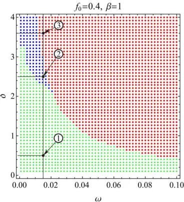
equal to unity (1), which corresponds to the case when the spring from Fig. A1 is compressed to the half of its undeformed length at the position O. Thus, by fixing f00.4 and varying the parameters  and , qualitatively different resulting behaviour is captured numerically and presented in Fig. 1. Depending on the combination of  and  , three characteristic motions can be detected, which are labelled by dots of different colour: the green dots are associated with bursting oscillations (their characteristics are explained in the Introduction); the blue dots represent relaxation oscillations (Rand 2012), consisting of slow motions along outer curves and fast changes of the amplitude (jumps); the red dots stand for oscillations around a non-trivial value.

Fig. 1. The -parametric plane with different behaviour plotted for f=0.4 and 1 (red dots - oscillations around a non-trivial value; blue dots - relaxation oscillations; green dots - bursting

oscillations)

To illustrate each of these responses, the excitation frequency is fixed at the value

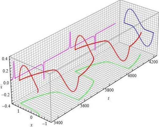
and three points corresponding to different  are labelled: Points 1 (, Point 2 (and Point 3 ( Figs. 2-4 show their 3D (txx) responses as well as 2D responses as time-response diagrams in the tx plane, phase trajectories in the xx plane and time-velocity diagrams in the tx plane. Note that in the case of bursting and relaxation oscillations (Figs. 2 and 3), the time-velocity diagrams show clearly that the velocity changes in such a way that periods of almost zero velocity are followed by sudden increases (peaks/bursters), which indicates that the corresponding motion is associated with slow motion followed by sudden changes of the amplitude (jumps), as illustrated by the green curves in Figs. 2 and 3. In the case of bursting oscillations, additional fast oscillations occur along the outer curves (see the green curve in Fig. 2).

qualitatively different, but the same behaviour – oscillations around non-trivial values. Given the structure and its features, this basin is similar to the one explained for Eq. (2).

Fig. 2. 3D and 2D representations of the response of Point 1 from Fig. 1: time-response in the

x

t plane, phase trajectory the in xx plane and time-velocity diagram in the tx plane.

Fig. 3. 3D and 2D representations of the response of Point 2 from Fig. 1: time-response in the

x

Fig. 4. 3D and 2D representations of the response of Point 3 from Fig. 1: time-response in the

x

t plane, phase trajectory the in xx plane and time-velocity diagram in the tx plane.

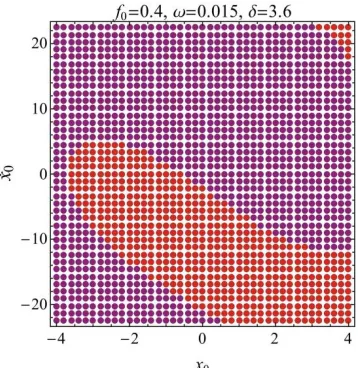
Fig. 5. Basin of attraction of Point 3 (red dots – oscillations around negative values of x, violet dots – oscillations around positive values of x).

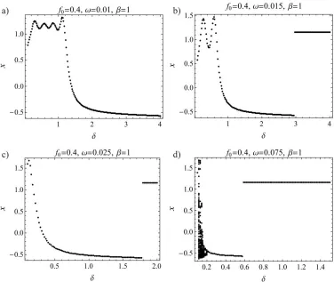
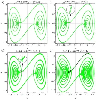
present the development of the response for decreasing values of  in the phase plane with Poincaré dots shown in black: for period-1 motion exists (Fig. 8a), while for  period-2 motion appears (Fig. 8b); when , the number of Poincaré points indicates period-3 motion, and for the Poincaré section shown indicates the possibility of chaotic response. Note that this approach gives the threshold value of the excitation representing the limit between small and non-small excitation frequencies as for the value shown in Fig. 6d the system starts behaving differently than in Figs. 6a-c, i.e. Figs. 2-4.

Fig. 7. The enlarged bifurcation diagrams from Fig. 6d.

Fig. 8. Phase trajectories and Poincaré sections for the case of decreasing : a) ; b)

3. Appearance of three characteristic response: parametric study

3.1 Influence of the angular frequency

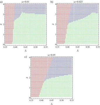
Another insight into this system’s behaviour is obtained by solving (3) numerically for the fixed value of the angular frequency  and for varying f0 and . The corresponding charts are presented in Fig. 9 for small and increasing values of . It is seen that oscillations around a non-zero value (red region) occur for smaller values of f0, and this region is almost vertical for

= 0.01, and inclines clockwise as increases. As in the -  plane, in this f0 - parametric plane, bursting oscillations (green region) appear for lower values of and relaxation oscillations (blue region) for higher values of . It should be pointed out that they cannot appear for any value of f0, and the threshold for the appearance of mixed-mode oscillations (bursting and relaxation) is defined by the right hand boundary of the red region.

Fig. 9. The f-parametric plane with different behaviour plotted for different values of : a)

3.2 Influence of the excitation magnitude

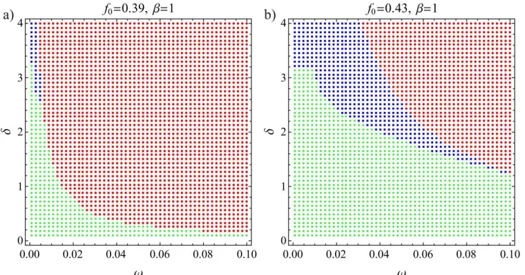
The parametric chart  with three distinctive regions presented in Fig. 1 is plotted for one specific value of f0. To determine how these regions change if the value of f0 decreases or increases, two more charts have been produced numerically and are presented in Fig. 10. In the former case, the regions of relaxation oscillations and bursting oscillations shrink, while in the latter case, the opposite is true. It is also noticeable that relaxation oscillations appear for high values of . Given the region of values studied, these charts do not clearly show what happens for very small values of  (those below 0.1) and this will be investigated in future studies.

Fig. 10. The parametric plane with characteristic responses indicated plotted for different values of f: a) f; b) f

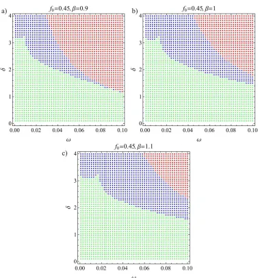
3.3 Influence of the coefficient of nonlinearity

Fig. 11. The -parametric plane with different behaviour plotted for different values of : a)

; b) ; c) .

4.Conclusions

with positive and negative values of the offset, and that damping directly controls the route to chaos through period-2 and period-3 motions as well as the transition between bursting and relaxation oscillations. It is also noted that the excitation amplitude directly drives the respective sizes of the bursting and relaxation regions in the parameter space and that the value of the coefficient of the nonlinear term directly influences the size of the region of mixed-mode oscillations. The effects of very low levels of damping remain to be explored and will form the focus of a future study.

Appendix. Mechanism and governing equation

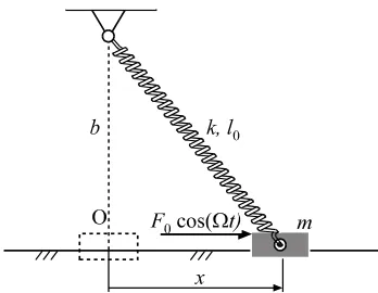
One of the simplest mechanisms which equation of motion has the form that can reasonably be approximated by Eq. (3) is shown in Fig. A1. It consists of a slider of mass m moving along a frictionless horizontal guide. The attached spring has a stiffness k and the length l0 when in the undeformed state. In the position O, when x = 0, the spring is compressed to the length b (note that l₀b). The horizontal force acting on the slider changes harmonically according to

t F

F ₀cos . It is assumed that the slider is lubricated by a viscous fluid so that the corresponding damping force is proportional to its velocity, with the damping coefficient c.

Fig. A1 Mechanical model of the oscillator under consideration

Thus, the kinetic energy, potential energy, dissipative force and the generalised force are, respectively, given by:





1 2 2

0 2 2 2 F Q x c l x b c V x m

T       x (A1)

Lagrange’s equation: , x Q x V x x T x T dt d _                     (A2)

with the potential term developed into series, yields:

 

0 _{x F t}

b l k x b l k x b b l k x c x

m        (A3)

Assuming that the quintic term is considerably smaller than the cubic one, i.e. 2 4 2/3

b

x 

also suitable here as the aim of the paper is not to get a definitively quantitative, but qualitative insight into the system dynamics.

After introducing the non-dimensional parameters





















and omitting the overbar, the equation of motion (A3) transforms into the following non-dimensional equation:

 

x    

 (A5)

Acknowledgements IK and MZ acknowledge financial support provided by the Ministry of Education, Science and Technological Development of the Republic of Serbia (Grant III 41007).

Извод

Одлике динамичког понашања двојних осцилатора са ниском

фреквенцијом побуђености: нумерички увиди

M. Zukovic1, I. Kovacic1,*, M. P. Cartmell2

1 _{Универзитет у Новом Саду, Факултет техничких наука, Центар изузетних вредности за} вибро-акустичке системе и обраду сигнала CEVAS, 21 000 Нови Сад, Србија

Email [email protected] Email [email protected] 2

References

Han X, Bi Q (2011). Bursting oscillations in Duffing’s equation with slowly changing external forcing, Communications in Nonlinear Sciences and Numerical Simulations, 16, 4146– 4152.

Holmes PJ (1979). A nonlinear oscillator with a strange attractor, Philosophical Transactions of the Royal Society of London A, 292, 419-448.

Kovacic I, Brennan MJ (2011). The Duffing Equation: Nonlinear Oscillators and their Behaviour. John Willey & Sons.

Kovacic I, Cartmell M, Zukovic M (2015). Mixed-mode dynamics of bistable oscillators with low-frequency excitation: behavioural mapping, approximations for motion and links with van der Pol oscillators, Proceedings of the Royal Society A, in press.

Lansbury AN, Thompson JMT, Stewart HB (1992). Basin erosion in the twin-well Duffing oscillator: Two distinct bifurcation scenarios. International Journal of Bifurcation and Chaos, 2, 505-532.

Moon FC, Holmes PJ (1979). A magnetoelastic strange attractor, Journal of Sound and Vibration, 65, 275-296.

Rand RH (2012). Lecture Notes in Nonlinear Vibrations, published online by the Internet–First University Press: http://ecommons.library.cornell.edu/handle/1813/28989.

Szemplinska-Stupnicka W (1992). Cross-well chaos and escape phenomena in driven oscillators, Nonlinear Dynamics, 3, 225-243.

Szemplinska-Stupnicka W, Janicki KL (1997). Basin boundary bifurcations and boundary crisis in the twin-well Duffing oscillator: Scenarios related to the saddle of the large resonant orbit. International Journal of Bifurcation and Chaos, 7, 129-146.

Szemplinska-Stupnicka W, Rudowski J (1993). Steady-states in the twin-well potential oscillator: Computer simulations and approximate analytical studies, Chaos – International Journal of Nonlinear Science, 3, 375-385.

Tseng WY, Dugundji J (1971). Nonlinear vibrations of a buckled beam under harmonic excitation, ASME Journal of Applied Mechanics, 38, 467-476.