Open Access
Research article
A simulation study comparing aberration detection algorithms for
syndromic surveillance
Michael L Jackson*
1,2, Atar Baer
1, Ian Painter
3and Jeff Duchin
1,2Address: 1Public Health – Seattle and King County, 999 Third Avenue, Suite 500, Seattle WA, 98104, USA, 2Department of Epidemiology,
University of Washington, Mail Box 357236, Seattle WA, 98195-7236, USA and 3Foundation for Healthcare Quality, 705 Second Avenue, Suite
703, Seattle WA, 98104, USA
Email: Michael L Jackson* - [email protected]; Atar Baer - [email protected]; Ian Painter - [email protected]; Jeff Duchin - [email protected]
* Corresponding author
Abstract
Background: The usefulness of syndromic surveillance for early outbreak detection depends in part on effective statistical aberration detection. However, few published studies have compared different detection algorithms on identical data. In the largest simulation study conducted to date, we compared the performance of six aberration detection algorithms on simulated outbreaks superimposed on authentic syndromic surveillance data.
Methods: We compared three control-chart-based statistics, two exponential weighted moving averages, and a generalized linear model. We simulated 310 unique outbreak signals, and added these to actual daily counts of four syndromes monitored by Public Health – Seattle and King County's syndromic surveillance system. We compared the sensitivity of the six algorithms at detecting these simulated outbreaks at a fixed alert rate of 0.01.
Results: Stratified by baseline or by outbreak distribution, duration, or size, the generalized linear model was more sensitive than the other algorithms and detected 54% (95% CI = 52%–56%) of the simulated epidemics when run at an alert rate of 0.01. However, all of the algorithms had poor sensitivity, particularly for outbreaks that did not begin with a surge of cases.
Conclusion: When tested on county-level data aggregated across age groups, these algorithms often did not perform well in detecting signals other than large, rapid increases in case counts relative to baseline levels.
Background
In the short time since syndromic surveillance[1] was introduced as an early warning system for detecting out-breaks, considerable effort and expense have gone into developing syndromic surveillance systems. Although there have been substantial developments in the methods and tools used for this practice, the public health value of the various approaches to syndromic surveillance has
rarely been evaluated. In particular, a critical component needing further study is the relative accuracy and timeli-ness of the aberration detection methods of these systems.
In aberration detection, statistical models determine whether the counts in a given syndrome and day are unu-sually high and thus worth investigating. Many statistical algorithms are available, including control-chart-based
Published: 1 March 2007
BMC Medical Informatics and Decision Making 2007, 7:6 doi:10.1186/1472-6947-7-6
Received: 6 December 2006 Accepted: 1 March 2007
This article is available from: http://www.biomedcentral.com/1472-6947/7/6
© 2007 Jackson et al; licensee BioMed Central Ltd.
models[2,3], scan statistics[4,5], autoregressive moving averages[6], and regression models[7,8]. To optimize out-break detection, surveillance system designers and users need to understand which methods perform well or poorly in different settings.
Many studies have described the performance of individ-ual aberration detection methods [3-10]. However, multi-ple algorithms have seldom been compared on the same data [11-14], which is problematic because algorithms that work well for one data source may not do as well for another. Further, studies comparing different algorithms have either tested the algorithms on only a single type of outbreak[11,14], or have used simulated baseline data rather than syndrome counts from real systems[12,13]. Using real system data is important, because it is unknown how well simulated data approximate the rele-vant features of real syndrome counts. Testing perform-ance on outbreaks of different temporal distributions and sizes is important because of the uncertainty about the types of outbreaks likely to be encountered in practice. To date, no published studies have systematically compared detection methods using real syndromic surveillance data. This lack of comparisons on actual syndromic surveillance data makes it difficult to select aberration detection meth-ods objectively.
To address these limitations, we compared the utility of six commonly-used aberration detection algorithms using data from our syndromic surveillance system at Public Health – Seattle & King County. We simulated syndrome counts that might result from a variety of outbreaks, and added these to actual daily counts from syndromes mon-itored by our system. We then evaluated the performance of the six algorithms on the resulting data.
Methods
Our syndromic surveillance system receives data from 18 of 19 emergency departments (EDs) in King County. Each morning, EDs send data on all visits that occurred the pre-vious day, including the date and time of the visit; the patient's age, sex, and home zip code; a free-text chief complaint; diagnosis, if available; and disposition. Chief complaints are classified into syndromes based on the presence or absence of key words using a modified version of the chief complaint coder developed by the New York City Department of Health and Mental Hygiene[15]. For each syndrome, daily case counts are determined both by age group and aggregated across age groups. In this study, we used the aggregated counts. Because historical data were not available from all EDs when we began this study, we restricted our analysis to the nine EDs with complete reporting from 2001–2004.
Because we could not use all of the syndromes we monitor in this analysis, we chose a representative set by grouping syndromes into four categories based on their mean daily counts, and then selecting one syndrome from each group. The final syndromes we used as baselines had mean (standard deviation) daily counts of 60 (16.0), 35 (9.9), 10 (4.0), and 2 (1.6) visits per day. These counts corresponded to ED visits for respiratory illness, influ-enza-like illness, and asthma syndromes, and pneumonia hospitalizations, respectively. From these four baselines we used data from 2001 through 2003 to provide back-ground counts for the algorithms, and used data from 2004 for testing the algorithms. For each of these syn-dromes, we calculated the variability in daily counts by weekday and month using Poisson regression [see Addi-tional file 1]. Notably, all four baselines had significant month effects, indicating the presence of seasonal trends. The four baselines also showed significant day-of-week effects.
We compared the performance of six aberration detection methods. We evaluated the three control-chart-based algorithms commonly referred to as C1, C2, and C3[13]. For C1 and C2, the test statistic on day t was calculated as
St = max(0, (Xt - (μt + k*σt))/σt)
where Xt is the count on day t, k is the shift from the mean to be detected, and μt and σt are the mean and standard deviation of the counts during the baseline period. For C1, the baseline period is (t-7,...,t-1); for C2 the baseline is (t-9,...,t-3). The test statistic for C3 is the sum of St + St-1 + St-2 from the C2 algorithm.
We evaluated a generalized linear model (GLM), using a three-year baseline and Poisson errors, with terms for day of the week, month, linear time trend, and holidays. The full model for the expected count on day t was
E(Xt) = β0 + β1(Sunday) + ... + β6(Friday) + β7(January) + ... + β17(November) + β18(Holiday) + β19(time trend)
and the test statistic was the probability from a Poisson distribution of observing at least Xt cases given E(Xt).
We also included two Exponential Weighted Moving Average (EWMA) models[16], using a 28-day baseline and smoothing constants of 0.4 (EWMA4) and 0.9 (EWMA9). The smoothed daily counts were calculated as
Y1 = X1; Yt = ω*Xt + (1 - ω)*Yt-1
and the test statistic was calculated as
where ω is the smoothing constant and other notation as defined above. The baseline period for μt and σt was set to (t-30,...,t-3).
Outbreak simulation
Rather than try to model the full outbreak process from infection to ED visit, as has been done for some limited outbreak types[17], we tried to model a wide range of out-break signals, representing various ways that outout-breaks in the community could alter ED syndrome counts. We based our simulations on the approach described by Mandl et al[18]. First, we chose five temporal distribu-tions, using the epidemic curves of historical outbreaks, to represent several ways in which a pathogen could spread through a community (Figure 1). These were (a) the air-borne release of a bioweapon[19]; (b) point-source expo-sure to an infectious agent[20]; (c) transmission of a pathogen spread by close contact;[21] (d) transmission of
an airborne pathogen[22]; and (e) transmission resulting in a multi-modal distribution[23]. Next, we simulated a range of outbreak signal durations (lasting 1, 2, 4, 6, 8, 16, and 32 days) and a range of sizes using the forecast errors of the six algorithms[18]. We determined the forecast errors for each algorithm for each day of 2004, and calcu-lated the standard deviations of these errors. We set the size of the largest outbreak signal to be roughly four times the largest standard deviation, rounded to a convenient number. The largest standard deviation was 13.2 counts, and our outbreak signals ranged from 5 to 50 cases in increments of 5.
Next, we simulated daily outbreak signal counts by creat-ing every unique combination of the temporal distribu-tions, duradistribu-tions, and sizes. Since all outbreaks of one day duration have the same temporal distribution, this gave us 310 different outbreak signals. For each signal, we
con-Temporal distributions used for simulating outbreaks, from the epidemic curves of historic outbreaks, with references Figure 1
verted the epidemic curve of the appropriate historical outbreak into an empirical probability distribution. We divided this distribution into the appropriate number of days for the simulated outbreak. We then calculated the cumulative probability of a case occurring on or before day d for each day (1,...,d) of the outbreak signal. Finally, we assigned each case a random number between 0 and 1, chosen from a uniform random distribution. The total number of cases on day d was the sum of all cases whose random number was greater than the cumulative proba-bility for day d-1, and less than or equal to the cumulative probability for day d. This random assignment was repeated for each of the 310 outbreak signals.
Algorithm testing
We created evaluation datasets by adding the simulated outbreak signals to each of the four baselines, with the outbreak counts starting on January 2nd, 2004. To avoid bias due to day-of-the-week effects and seasonality, we repeated this process starting the outbreak on every other day of 2004 for each of the four baselines. This gave us 183 datasets per outbreak per baseline, for a total of 226,920 datasets for analysis.
We applied the six algorithms to the evaluation datasets, and calculated two outcome measures for each algorithm on each dataset. The first was whether the algorithm ever detected the outbreak signal. The second was the earliest day of an alert, among signals that were detected. The ear-liest day of alert was counted from the day on which the first simulated case was added. Due to the stochastic nature of these simulations, this was not always the first day of the epidemic. For example, consider a simulated outbreak signal of five cases 32 days duration started on January 2nd, 2004. The cases might appear on days 3, 5, 8,
17, and 30 of the signal. In this situation, we would begin counting the days until detection starting from day 3 (Jan-uary 4th).
We calculated these outcomes while running the algo-rithms at an alert rate of 0.01 (an average of one alert every hundred days). We set this alert rate empirically by apply-ing each algorithm to each baseline without any added outbreak signals, and determining the threshold that would yield an average of one alert per 100 days. Note that in this study we defined an alert rate, rather than a false positive rate (which is 1 – specificity). Calculating a false positive rate (i.e. a specificity) requires assuming that the baseline syndromes did not contain any signals from true outbreaks in the community. This is an unreasonable assumption, given the known yearly influenza epidemics and the probable presence of other unknown outbreaks. By using an alert rate instead of a false positive rate, we allowed for the existence of these signals in our baseline data.
Comparing algorithm performance
For each of the 310 outbreak signals, in each of the four baseline syndromes, we computed the sensitivity (that is, the probability of detecting the signal given the presence of an outbreak) by averaging the detection outcome across all 183 analysis runs. We also computed the median of the earliest day of detection. We used ANOVA to test for significant differences in the algorithms' sensi-tivities. Separate tests were conducted by baseline and by outbreak distribution, duration, and size. In each stratum of these four grouping variables we tested for significant differences between algorithms in the probability of detection. We also tested for differences within each algo-rithm across the strata. For all ANOVA comparisons that were significant at the 0.05 level, we compared the per-formance of all pairs of algorithms by t-test.
We also present a figure showing the performance of one algorithm on each of the 310 simulated outbreak signals, at each of the four baselines. Because of the multiple com-parisons problem, we did not test for significant differ-ences between the cells of the figure. However, we present this figure for qualitative comparisons, so that the reader can visualize the effects of baseline and outbreak temporal distribution, size, and duration on relative algorithm per-formance, over the range of outbreak signals we tested (Figure 2). All simulations and analyses were performed using SAS version 8.2 (SAS Institute Inc., Cary North Caro-lina).
Results
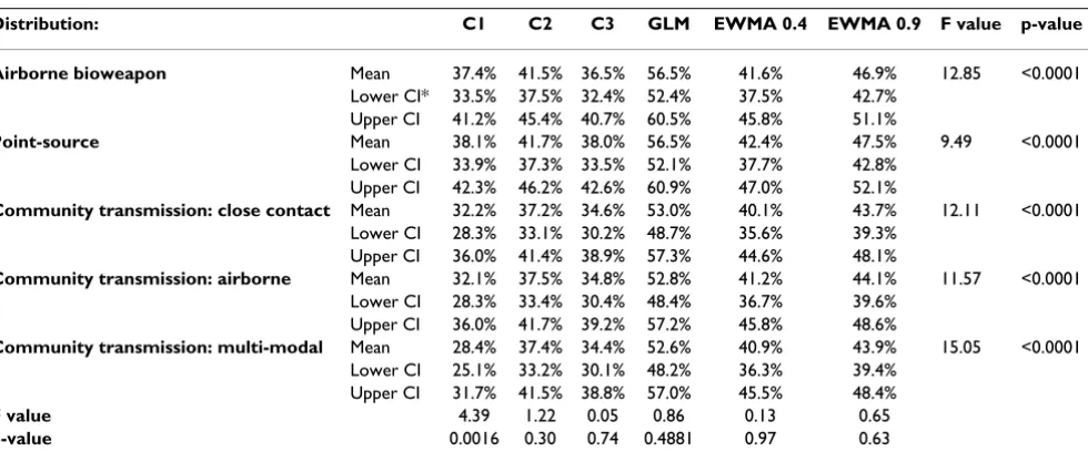
Of the algorithms evaluated, only the performance of C1 varied across outbreak distributions (p = 0.002) (Table 2). C1 had better detection for the point-source distribution (mean probability of detection 38.1%) compared with the three community-transmission distributions (p < 0.05 for all pairwise t-tests). Although the other algorithms had similar patterns of detection, the differences were not sig-nificant at the 0.05 level. Within each outbreak distribu-tion, the GLM had better detection compared with the other algorithms (p < 0.0001 comparing GLM to C1, C2, or C3; p < 0.01 comparing the GLM to EWMA4 and EWMA9), with sensitivities as high as 56.5% for both the airborne bioweapon and the point-source distributions. The sensitivities of the two EWMA models did not differ across distributions (p > 0.05 for all comparison).
Across all six algorithms, the probability of detection increased as the size of the outbreak increased (Table 3). Within each outbreak size, GLM had better detection than
the other algorithms (p < 0.001 comparing GLM to C1, C2, or C3; p < 0.05 comparing GLM to EWMA4 or EWMA9). The probability of detection tended to be low for all six algorithms even at the largest outbreak sizes (50 extra cases above the baseline), ranging from 52.9% for C1 (95% CI = 47.0%–58.7%) to 77.4% with GLM (95% CI = 72.9%–81.9%).
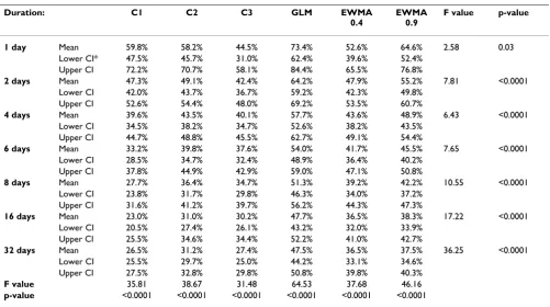
Outbreak duration was inversely related to sensitivity for all algorithms (Table 4). The probability of detection was highest for one- and two-day surges in cases. However, even when all excess cases occurred on a single day, detec-tion was fairly poor for most algorithms, ranging as low as 44.5% with C3 (95% CI = 31.0%–58.1%). The GLM was better than all other algorithms at detecting single-day surges in cases (73.4%, 95% CI = 62.4%–84.4%), with the exception of EWMA9, where the difference between the two methods was not significant (p < 0.05). Within each of the other categories of outbreak duration, the GLM had
Guide to interpreting Figure 3 Figure 2
Guide to interpreting Figure 3.
1 day
568 26 29 26 22 30 43 26 22 21 24 22 34 10100 98 96 74 56 54 51 85 55 48 44 37 42 15100 100 100 90 84 73 58 100 95 73 76 76 53 20100 100 100 100 96 91 67 100 100 96 91 88 60 25100 100 100 100 100 98 74 100 100 100 99 99 72 30100 100 100 100 100 98 76 100 100 100 99 99 96 35100 100 100 100 100 100 85 100 100 100 99 99 97 40100 100 100 100 100 100 91 100 100 100 99 99 97 45100 100 100 100 100 100 95 100 100 100 99 99 98 50100 100 100 100 100 100 98 100 100 100 100 99 98
5 1 4 6 7 10 16 28 4 7 7 9 13 19 10 4 6 8 9 10 19 30 6 8 10 10 16 21 1511 9 9 12 11 20 30 12 12 11 13 16 22 2028 14 14 14 14 20 31 17 14 15 15 18 25 2545 23 21 17 19 22 31 26 18 20 18 19 26 3060 38 24 21 20 22 32 38 23 25 24 22 28 3573 49 26 25 22 24 34 54 32 30 26 22 29 4084 62 40 30 26 27 34 63 45 38 29 24 29 4591 67 48 32 30 29 35 71 52 41 32 25 30 5095 78 58 38 33 34 37 77 58 51 34 29 31 1 2 4 6 8 16 32 2 4 6 8 16 32
0.8 - 1.0 0.6 - 0.79 0.4 - 0.59 0.2 - 0.39 0 - 0.19
Median day of first alert, among detected outbreaks First day Second day Third day After third day Legend
Probability of detecting the outbreak Distribution 60 2 Si m u la te d out br eak si gnal : addi ti onal count s above basel in e
Number of days over which outbreak signal counts are spread
Aver age dai ly count s of basel in e Community transmission: Multi-modal Airborne bioweapon
Major columns show the five distributions, plus a column for single-day outbreaks.
Minor rows indicate the total number of cases added to the baseline from the simulated outbreak signal.
Minor columns show the duration of the simulated outbreak signal.
Major rows indicate the baselines, by average daily counts.
better detection than the other algorithms (p < 0.001 comparing GLM to C1, C2, or C3; p < 0.05 comparing GLM to EWMA4 or EWMA9).
Because the GLM generally detected more outbreaks than the other algorithms when stratified by outbreak size, duration, distribution, or baseline, we present a more detailed view of this algorithm stratified by these four fac-tors simultaneously (Figure 3). As described in Figure 2, each cell in this figure shows the probability of detecting an outbreak for different outbreak signals. To allow for quick qualitative comparisons across outbreak character-istics, the cells are color-coded and shaded, with colors indicating the median day of the first alert among detected
outbreaks, and darker shades indicating a higher likeli-hood of detection.
This stratification suggests several qualitative trends. First, regardless of distribution, the GLM tended to have low sensitivity when the baseline counts for a given syndrome were 35 per day or higher. As shown in Figure 3, outbreak detection under these circumstances was generally below 80%, except in some situations where the outbreak size was large relative to the baseline (i.e., 35–40 excess counts per day) and the surge in cases occurred on a single day. For example, a single-day surge of influenza-like illness resulting in 35 cases above the average daily baseline count of 35 cases was detected in 84% of the tests. That is, a doubling of the average daily case counts on a single day
Table 2: Mean percent of outbreak signals detected by six aberration detection algorithms, tested on five outbreak distributions, at an alert rate of 0.01
Distribution: C1 C2 C3 GLM EWMA 0.4 EWMA 0.9 F value p-value
Airborne bioweapon Mean 37.4% 41.5% 36.5% 56.5% 41.6% 46.9% 12.85 <0.0001
Lower CI* 33.5% 37.5% 32.4% 52.4% 37.5% 42.7% Upper CI 41.2% 45.4% 40.7% 60.5% 45.8% 51.1%
Point-source Mean 38.1% 41.7% 38.0% 56.5% 42.4% 47.5% 9.49 <0.0001
Lower CI 33.9% 37.3% 33.5% 52.1% 37.7% 42.8% Upper CI 42.3% 46.2% 42.6% 60.9% 47.0% 52.1%
Community transmission: close contact Mean 32.2% 37.2% 34.6% 53.0% 40.1% 43.7% 12.11 <0.0001
Lower CI 28.3% 33.1% 30.2% 48.7% 35.6% 39.3% Upper CI 36.0% 41.4% 38.9% 57.3% 44.6% 48.1%
Community transmission: airborne Mean 32.1% 37.5% 34.8% 52.8% 41.2% 44.1% 11.57 <0.0001
Lower CI 28.3% 33.4% 30.4% 48.4% 36.7% 39.6% Upper CI 36.0% 41.7% 39.2% 57.2% 45.8% 48.6%
Community transmission: multi-modal Mean 28.4% 37.4% 34.4% 52.6% 40.9% 43.9% 15.05 <0.0001
Lower CI 25.1% 33.2% 30.1% 48.2% 36.3% 39.4% Upper CI 31.7% 41.5% 38.8% 57.0% 45.5% 48.4%
F value 4.39 1.22 0.05 0.86 0.13 0.65
p-value 0.0016 0.30 0.74 0.4881 0.97 0.63
* CI = 95% confidence interval
Table 1: Mean percent of outbreak signals detected by six aberration detection algorithms, tested on four baseline syndromes, at an alert rate of 0.01
Syndrome: C1 C2 C3 GLM EWMA 0.4 EWMA 0.9 F value p-value
Pneumonia hospitalizations (mean 2 visits per day) Mean 62.0% 69.3% 72.0% 85.3% 80.5% 79.6% 24.94 <0.0001
Lower CI* 58.3% 65.8% 68.6% 82.5% 77.2% 76.3%
Upper CI 65.8% 72.9% 75.5% 88.0% 83.9% 82.9%
Asthma visits (mean 10 visits per day) Mean 35.4% 52.2% 48.8% 70.0% 52.3% 57.7% 36.63 <0.0001
Lower CI 31.7% 48.5% 45.1% 66.5% 48.6% 53.9%
Upper CI 39.0% 56.0% 52.5% 73.4% 56.0% 61.5%
Influenza-like illness visits (mean 35 visits per day) Mean 21.2% 17.9% 11.1% 34.4% 19.0% 28.2% 84.08 <0.0001
Lower CI 19.6% 16.5% 10.4% 31.9% 17.4% 26.0%
Upper CI 22.9% 19.2% 11.9% 36.9% 20.5% 30.4%
Respiratory visits (mean 60 visits per day) Mean 16.4% 17.1% 10.8% 27.8% 13.3% 15.7% 84.90 <0.0001
Lower CI 15.1% 16.0% 10.3% 25.7% 12.5% 14.5%
Upper CI 17.6% 18.3% 11.4% 29.8% 14.0% 16.9%
F value 205.58 349.50 531.70 398.73 550.30 406.76
p-value <0.0001 <0.0001 <0.0001 <0.0001 <0.0001 <0.0001
could be reliably detected 84% of the time. This detection level dropped to 55–74% (depending on the distribution)
if the excess counts were spread over a period of two days. Sensitivity was poorer with smaller outbreak sizes. For
Table 3: Mean percent of outbreak signals detected by six aberration detection algorithms, tested on six outbreak sizes, at an alert rate of 0.01
Size: C1 C2 C3 GLM EWMA
0.4
EWMA 0.9
F value p-value
5 cases Mean 10.4% 11.9% 9.6% 16.0% 10.3% 12.0% 9.55 <0.0001
Lower CI* 8.9% 10.5% 8.3% 14.1% 9.0% 10.6% Upper CI 11.8% 13.3% 10.9% 18.0% 11.7% 13.5%
10 cases Mean 16.4% 18.8% 15.4% 30.2% 20.2% 22.9% 10.01 <0.0001
Lower CI 13.7% 16.2% 13.0% 25.7% 16.7% 19.0% Upper CI 19.2% 21.5% 17.9% 34.6% 23.8% 26.7%
20 cases Mean 26.7% 32.2% 29.4% 48.4% 34.8% 38.4% 8.17 <0.0001
Lower CI 22.1% 27.3% 24.3% 42.5% 29.0% 32.7% Upper CI 31.3% 37.2% 34.5% 54.3% 40.6% 44.2%
30 cases Mean 38.9% 46.2% 42.5% 63.0% 47.8% 52.5% 7.42 <0.0001
Lower CI 33.3% 40.0% 36.0% 57.2% 41.3% 46.1% Upper CI 44.5% 52.4% 49.0% 68.7% 54.3% 58.9%
40 cases Mean 47.1% 53.7% 50.0% 71.6% 56.4% 61.6% 8.11 <0.0001
Lower CI 41.2% 47.4% 43.2% 66.6% 49.8% 55.4% Upper CI 53.0% 59.9% 56.9% 76.6% 63.0% 67.7%
50 cases Mean 52.9% 58.8% 53.8% 77.4% 62.7% 67.9% 9.83 <0.0001
Lower CI 47.0% 52.8% 47.0% 72.9% 56.5% 62.2% Upper CI 58.7% 64.8% 60.6% 81.9% 68.9% 73.7%
F value 35.81 38.67 31.48 64.53 37.68 46.16
p-value <0.0001 <0.0001 <0.0001 <0.0001 <0.0001 <0.0001
* CI = 95% confidence interval
Table 4: Mean percent of outbreak signals detected by six aberration detection algorithms, tested on seven outbreak durations, at an alert rate of 0.01
Duration: C1 C2 C3 GLM EWMA
0.4
EWMA 0.9
F value p-value
1 day Mean 59.8% 58.2% 44.5% 73.4% 52.6% 64.6% 2.58 0.03
Lower CI* 47.5% 45.7% 31.0% 62.4% 39.6% 52.4% Upper CI 72.2% 70.7% 58.1% 84.4% 65.5% 76.8%
2 days Mean 47.3% 49.1% 42.4% 64.2% 47.9% 55.2% 7.81 <0.0001
Lower CI 42.0% 43.7% 36.7% 59.2% 42.3% 49.8% Upper CI 52.6% 54.4% 48.0% 69.2% 53.5% 60.7%
4 days Mean 39.6% 43.5% 40.1% 57.7% 43.6% 48.9% 6.43 <0.0001
Lower CI 34.5% 38.2% 34.7% 52.6% 38.2% 43.5% Upper CI 44.7% 48.8% 45.5% 62.7% 49.1% 54.4%
6 days Mean 33.2% 39.8% 37.6% 54.0% 41.7% 45.5% 7.65 <0.0001
Lower CI 28.5% 34.7% 32.4% 48.9% 36.4% 40.2% Upper CI 37.8% 44.9% 42.9% 59.0% 47.1% 50.8%
8 days Mean 27.7% 36.4% 34.7% 51.3% 39.2% 42.2% 10.55 <0.0001
Lower CI 23.8% 31.7% 29.8% 46.3% 34.0% 37.2% Upper CI 31.6% 41.2% 39.7% 56.2% 44.3% 47.3%
16 days Mean 23.0% 31.0% 30.2% 47.7% 36.5% 38.3% 17.22 <0.0001
Lower CI 20.5% 27.4% 26.1% 43.2% 32.0% 33.9% Upper CI 25.5% 34.6% 34.4% 52.2% 41.0% 42.7%
32 days Mean 26.5% 31.2% 27.4% 47.5% 36.5% 37.5% 36.25 <0.0001
Lower CI 25.5% 29.7% 25.0% 44.2% 33.1% 34.6% Upper CI 27.5% 32.8% 29.8% 50.8% 39.8% 40.3%
F value 35.81 38.67 31.48 64.53 37.68 46.16
p-value <0.0001 <0.0001 <0.0001 <0.0001 <0.0001 <0.0001
example, a single-day surge of 20 cases of influenza-like illness (a 57% increase over the mean baseline count of 35 cases per day) was detected in less than half (46%) of the tests.
Second, the GLM's performance was generally better for situations where the average daily baseline count was lower (i.e., 10 or fewer cases). In this scenario, the algo-rithm tended to detect the surge in cases within the first or second day with high probability (>80%). The probability
Percent of outbreak signals detected, and median timeliness of detection, for the generalized linear model running at an alert rate of 0.01, for each of 310 outbreak signals on each of four baseline syndromes
Figure 3
Percent of outbreak signals detected, and median timeliness of detection, for the generalized linear model running at an alert rate of 0.01, for each of 310 outbreak signals on each of four baseline syndromes.
1 day
5 68 26 29 26 22 30 43 26 24 24 26 26 31 26 24 23 26 34 34 55 26 22 17 19 25 26 22 21 24 22 34
10100 98 96 74 56 54 51 98 95 86 85 42 43 98 63 55 41 46 48 99 75 46 43 38 42 85 55 48 44 37 42
15100 100 100 90 84 73 58 100 100 100 99 59 52 100 87 81 60 57 59 99 96 89 65 56 54 100 95 73 76 76 53
20100 100 100 100 96 91 67 100 100 100 99 83 71 100 99 99 92 88 62 99 100 98 91 69 58 100 100 96 91 88 60
25100 100 100 100 100 98 74 100 100 100 99 99 85 100 99 100 100 98 73 99 100 99 99 90 66 100 100 100 99 99 72
30100 100 100 100 100 98 76 100 100 100 99 99 97 100 99 100 100 99 89 99 100 99 99 99 81 100 100 100 99 99 96
35100 100 100 100 100 100 85 100 100 100 99 99 99 100 99 100 100 99 98 99 100 99 99 99 90 100 100 100 99 99 97
40100 100 100 100 100 100 91 100 100 100 99 99 99 100 99 100 100 99 97 99 100 99 99 99 93 100 100 100 99 99 97
45100 100 100 100 100 100 95 100 100 100 99 99 99 100 99 100 100 99 99 99 100 99 99 99 94 100 100 100 99 99 98
50100 100 100 100 100 100 98 100 100 100 99 99 99 100 99 100 100 99 99 99 100 99 99 99 97 100 100 100 100 99 98
5 17 10 13 15 15 24 36 10 11 13 13 19 27 10 11 15 15 21 29 16 10 10 12 16 21 11 10 11 12 16 30
10 70 40 42 25 25 32 39 40 35 32 31 28 34 40 26 25 21 29 35 49 24 20 22 23 29 31 23 20 19 23 37
15 98 65 63 37 39 40 43 65 64 52 55 33 39 65 37 35 29 34 41 84 45 39 32 32 33 73 44 33 32 34 39
20100 92 90 65 54 46 49 92 85 84 80 43 46 92 74 59 47 45 43 99 75 56 45 37 38 92 66 50 45 46 42
25100 100 99 84 80 54 51 99 98 99 97 61 51 100 96 90 70 60 48 99 96 84 77 49 44 99 92 84 64 62 49
30100 100 100 96 84 63 54 100 100 100 99 83 61 100 99 100 89 72 57 99 100 99 92 69 53 99 100 96 88 92 65
35100 100 100 98 91 70 57 100 100 100 99 92 69 100 99 100 95 76 65 99 100 99 98 78 59 99 100 100 95 96 74
40100 100 100 100 97 83 63 100 100 100 99 98 81 100 99 100 99 90 68 99 100 99 99 90 65 99 100 100 98 100 77
45100 100 100 100 98 88 68 100 100 100 99 99 82 100 99 100 100 93 71 99 100 99 99 92 69 99 100 100 99 100 79
50100 100 100 100 99 97 74 100 100 100 99 99 91 100 99 100 100 96 79 99 100 99 99 97 74 99 100 100 99 100 84
5 4 5 7 8 10 17 33 5 4 7 6 12 23 5 4 5 8 12 27 3 5 5 6 10 17 4 5 7 7 12 23
10 11 10 11 11 12 18 34 10 8 10 10 14 26 10 7 8 9 14 30 9 8 8 8 13 25 8 7 8 9 13 25
15 27 14 15 13 14 18 35 14 12 14 13 15 26 14 11 10 9 15 30 23 11 12 10 13 26 16 10 10 11 16 28
20 46 23 20 17 17 21 35 21 24 19 21 18 26 23 19 16 13 18 30 40 16 14 15 16 26 28 15 14 13 17 28
25 59 42 34 21 23 23 37 34 38 31 37 22 28 42 36 23 18 21 32 55 25 22 21 19 28 42 21 21 16 21 29
30 73 53 38 30 27 26 37 49 48 45 48 28 30 53 47 36 26 23 32 64 38 35 32 23 29 55 38 33 29 26 31
35 84 61 44 34 32 28 39 55 55 53 53 34 32 58 55 43 32 27 33 74 48 46 42 27 30 64 48 44 35 34 33
40 90 74 54 44 43 32 41 66 64 65 64 45 34 72 63 54 40 34 36 84 57 53 48 33 31 72 58 53 42 38 35
45 96 78 58 47 45 35 41 73 68 69 68 48 37 77 67 57 43 39 38 95 62 59 53 36 33 80 64 57 46 41 38
50 98 88 72 55 50 42 44 83 79 77 75 51 38 87 74 65 51 41 41 98 70 66 60 42 33 86 72 62 47 47 40
5 1 4 6 7 10 16 28 4 7 5 8 11 20 4 7 7 7 12 26 6 4 7 7 10 19 4 7 7 9 13 19
10 4 6 8 9 10 19 30 6 10 9 10 14 25 6 9 8 12 15 31 9 8 8 9 16 26 6 8 10 10 16 21
15 11 9 9 12 11 20 30 9 13 10 12 15 26 9 9 11 12 17 31 15 11 10 9 15 28 12 12 11 13 16 22
20 28 14 14 14 14 20 31 14 18 12 15 16 27 14 14 13 14 18 31 24 15 13 11 16 28 17 14 15 15 18 25
25 45 23 21 17 19 22 31 20 26 17 21 18 28 23 22 15 17 22 32 38 18 15 16 18 28 26 18 20 18 19 26
30 60 38 24 21 20 22 32 33 32 28 29 23 29 38 28 20 21 24 33 54 23 20 21 21 29 38 23 25 24 22 28
35 73 49 26 25 22 24 34 42 40 35 37 25 30 46 37 25 25 24 34 63 30 28 24 22 30 54 32 30 26 22 29
40 84 62 40 30 26 27 34 55 55 52 52 31 31 58 52 38 29 27 34 75 44 38 29 24 31 63 45 38 29 24 29
45 91 67 48 32 30 29 35 61 60 57 57 32 33 64 56 43 32 30 34 85 51 45 31 26 31 71 52 41 32 25 30
50 95 78 58 38 33 34 37 72 70 66 63 34 36 76 63 52 36 31 36 93 60 52 40 29 32 77 58 51 34 29 31 1 2 4 6 8 16 32 2 4 6 8 16 32 2 4 6 8 16 32 2 4 6 8 16 32 2 4 6 8 16 32
Community transmission:
airborne
Community transmission:
Multi-modal Distribution
Airborne bioweapon Point source
Community transmission: close
contact
Aver
age dai
ly
count
s of
basel
in
e
10
35
Number of days over which outbreak signal counts are spread
60
Si
m
u
la
te
d out
br
eak si
gnal
: addi
ti
onal
count
s above basel
in
e
of detection was directly related to outbreak size and inversely related to outbreak duration.
Third, there were some qualitative differences in detection according to outbreak distribution. Distributions where the bulk of the cases occurred early (such as the airborne bioweapon) tended to be detected earlier than slowly-building outbreaks (such as the multi-modal community transmission).
Discussion
Although public health departments have been quick to adopt syndromic surveillance systems for outbreak detec-tion, few studies have demonstrated system effectiveness. The practical utility of syndromic surveillance depends on several factors, including the quality and accuracy of the source data; the sensitivity, specificity, predictive value, and timeliness of the aberration detection methods; and the user's response to alerts given by the system. In this study, we compared the performance of six aberration detection methods under a broad set of circumstances by adding simulated outbreak signals to actual daily syn-drome counts. To our knowledge, this is the largest simu-lation study comparing syndromic surveillance algorithms that has been published to date. Our evalua-tion was based on 310 unique outbreak signals, each of which was tested on 183 separate dates in each of four baselines.
Consistent with previous evaluations of syndromic sur-veillance algorithms[10,12,24], we found that the ability to detect outbreaks was better with larger outbreaks and lower baseline counts. We also observed that detection of a signal of a fixed size increases as the baseline counts decrease, which has been observed elsewhere[13]. This is unsurprising, as a fixed signal size causes a greater relative increase in the case count for a baseline with few daily cases compared to a baseline with many daily cases. Fur-thermore, our findings suggest that the temporal distribu-tion of cases (i.e., the shape of the epidemic curve) generally does not affect sensitivity but may affect timeli-ness, which Wang et al. observed in evaluating an autore-gressive periodic model (APM)[10].
Beyond these general observations, we had two more spe-cific findings. First, across different baselines, and differ-ent characteristics of the outbreak signals, the generalized linear model detected more outbreak signals than the other five algorithms. This was surprising, as we had expected to observe more heterogeneity in the relative per-formance of the algorithms, particularly across outbreak distributions. Buckeridge et al[25] have suggested that EWMA9 (which approximates a Shewhart chart) should outperform EWMA4 on single-day spikes and scattered signals (such as the multi-modal community
transmis-sion), while EWMA4 should be better on lognormal curves that increase rapidly (such as the close-contact community transmission). Furthermore, the control-chart-based methods have been reported to have good sensitivity for detection in rare syndromes, with C3 better suited than C1 and C2 for detecting slowly building out-breaks[13]. Of note, our baseline syndromes all had strong day-of-week trends [see Appendix]; since the GLM included weekday parameters, this may have contributed to its superior performance relative to the other methods, which do not correct for such trends[7].
Secondly, although we found that the GLM tended to form better than the other methods, all six algorithms per-formed poorly in many outbreak scenarios. The algorithms were generally able to detect large one- or two-day surges in case counts (where "large" means exceeding twice or three times the standard deviation of the base-line), or signals of longer duration that were very large rel-ative to the baseline. However, these are the types of signals most likely to be detected by the astute clinician (in the case of outpatient or ED data) or by an epidemiol-ogist visually looking for jumps in counts or proportions in a time series. Aberration detection is most needed for detecting low-to-moderate increases in cases and for slowly increasing outbreaks. Yet when run at a rate of one alert per 100 days, none of the algorithms we tested detected these types of signals reliably, suggesting that users run a high risk of missing outbreaks of interest across a wide range of scenarios.
One feature of Figure 3 deserves mention here. As the duration of the signal increases, sensitivity appears to fol-low either a U-shaped trend (when sensitivity is high in the early days of the outbreak) or to increase with increas-ing duration. At first glance, this is counter-intuitive, as the ability to detect a signal of a given size should decrease as the cases are distributed over more days. In this case, the superior sensitivity for longer outbreaks does not rep-resent a real benefit, but rather reflects the fact that there is a set alert rate of 0.01. An alert unrelated to the presence of a simulated outbreak, due to variation in the baseline syndrome counts, will occur roughly once every hundred days. It is more likely that such an alert will happen by chance during a simulated signal when that signal occurs over the course of 32 days than when the signal occurs over the course of one or two days.
wide array of the outbreak signals that could occur in prac-tice. Thus, our results may not be generalizable to all out-break settings, because the scenarios we produced may not be entirely representative of the scenarios for which the algorithms were designed to operate[26]. In addition, we set the alert rates for each algorithm empirically, by applying the algorithms to the baseline syndromes and finding the threshold that would yield approximately one alert every 100 days. The sensitivity of the algorithms used in this analysis will likely differ if those same algorithms are applied in systems that use different thresholds. Fur-thermore, the thresholds that gave an alert rate of 0.01 in our data may yield different alert rates in other data, and may also differ when applied to stratifications of the data, such as by age categories or geographic groupings.
It is a limitation of the syndromic surveillance literature that each evaluation has used different baseline data. The baselines likely differ in terms of random and systematic variation. Furthermore, published studies have rarely reported detailed information about their baseline time series; often, studies have not even reported mean counts or variances. This limitation makes comparisons between studies difficult and extrapolation to other datasets uncer-tain. We included the appendix, with its detail about the syndromes we used, primarily so that our baselines can be compared with other time series, at least in terms of mean counts, day-of-week effects, and seasonal trends. This gives other users a better basis for comparing our baseline counts with their own syndromic data. However, there may be other features of syndromic time series that affect algorithm performance. The field of syndromic surveil-lance would greatly benefit from an analysis of the fea-tures of syndromic time series that impact detection, and the relative importance of these features.
The poor overall performance of the algorithms we exam-ined raises another question: Are there other algorithms that may perform better? Because this study was computa-tionally intensive, we did not evaluate other algorithms that have been proposed for syndromic surveillance, such as autoregressive models[6,24] or the Pulsar method[11]. We were also unable to evaluate scan statistics[4,5] or other methods that use spatial data, because our simula-tion method aggregated cases to the county level. Com-paring our results to prior studies is difficult, not only because of the different baselines as mentioned above, but because studies have varied in the alert rates at which they have tested the algorithms. Prior studies have tended to use rates between 0.05 (one alert every 20 days) and 0.03 (roughly one alert per month). We feel that these rates are too high for routine surveillance and could desensitize users, leading to a reduced likelihood of following up on any given alert[27]. Because of the problems in comparing evaluations of algorithms across data sets, it is difficult to
determine whether other algorithms might have per-formed better on our data. This remains an area for active research.
Conclusion
The results of this study suggest that commonly-used aberration detection methods for syndromic surveillance often do not perform well in detecting signals other than large, rapid increases in case counts relative to baseline levels. To the degree that our results are generalizable to other settings, this poor performance may be a feature of other systems as well. These results suggest that users should exercise some caution in reviewing algorithm out-put. Although the GLM method tended to have better sen-sitivity overall, there was variability in algorithm performance across outbreak feature sets, illustrating that a one-size-fits-all method is unlikely. Additional work is still needed to develop and evaluate syndromic surveil-lance algorithms across outbreak signals and to determine the value of these systems in public health practice.
Competing interests
The author(s) declare that they have no competing inter-ests.
Authors' contributions
MLJ designed the study, programmed the simulations and analyses, and drafted the manuscript. AB helped conceive the study, was responsible for the data collection, helped design and coordinate the study, and helped draft the manuscript. IP participated in the design of the study and in programming the analyses. JD helped conceive and design the study and draft the manuscript. All authors have read and approved the final manuscript.
Additional material
Acknowledgements
This research is funded by the Centers for Disease Control and Prevention through a grant for Public Health Emergency Preparedness and Response, Focus Area B, Federal Catalogue Number 93.283. The funding agency did not contribute to the design or conduct of the study, the drafting of the manuscript, or the decision to publish.
Additional file 1
Appendix. This appendix contains results of Poisson regression analyses on the daily visit counts from the four syndrome time series used in this study. Click here for file
Publish with BioMed Central and every scientist can read your work free of charge "BioMed Central will be the most significant development for disseminating the results of biomedical researc h in our lifetime."
Sir Paul Nurse, Cancer Research UK
Your research papers will be:
available free of charge to the entire biomedical community
peer reviewed and published immediately upon acceptance
cited in PubMed and archived on PubMed Central
yours — you keep the copyright
Submit your manuscript here:
http://www.biomedcentral.com/info/publishing_adv.asp
BioMedcentral
References
1. Henning KJ: Appendix B: Syndromic Surveillance. In Institute of Medicine, 2003. Microbial Threats to Health: Emergence, Detection, and Response Edited by: Hamburg MA, Lederberg J. Washington, DC, The National Academies Press; 2003:309-350.
2. Hutwagner L, Thompson W, Seeman GM, Treadwell T: The bioter-rorism preparedness and response Early Aberration Report-ing System (EARS). J Urban Health 2003, 80:i89-96.
3. Rossi G, Lampugnani L, Marchi M: An approximate CUSUM pro-cedure for surveillance of health events. Stat Med 1999, 18:2111-2122.
4. Kleinman KP, Abrams AM, Kulldorff M, Platt R: A model-adjusted space-time scan statistic with an application to syndromic surveillance. Epidemiol Infect 2005, 133:409-419.
5. Kulldorff M, Heffernan R, Hartman J, Assuncao R, Mostashari F: A space-time permutation scan statistic for disease outbreak detection. PLoS Med 2005, 2:e59.
6. Miller B, Kassenborg H, Dunsmuir W, Griffith J, Hadidi M, Nordin JD, Danila R: Syndromic surveillance for influenzalike illness in ambulatory care network. Emerg Infect Dis 2004, 10:1806-1811. 7. Kleinman K, Lazarus R, Platt R: A generalized linear mixed
mod-els approach for detecting incident clusters of disease in small areas, with an application to biological terrorism. Am J Epidemiol 2004, 159:217-224.
8. Lazarus R, Kleinman K, Dashevsky I, Adams C, Kludt P, DeMaria A, Platt R: Use of automated ambulatory-care encounter records for detection of acute illness clusters, including potential bioterrorism events. Emerg Infect Dis 2002, 8:753-760. 9. Olson KL, Bonetti M, Pagano M, Mandl KD: Real time spatial clus-ter detection using inclus-terpoint distances among precise patient locations. BMC Med Inform Decis Mak 2005, 5:19. 10. Wang L, Ramoni MF, Mandl KD, Sebastiani P: Factors affecting
automated syndromic surveillance. Artif Intell Med 2005, 34:269-278.
11. Dafni UG, Tsiodras S, Panagiotakos D, Gkolfinopoulou K, Kouvatseas G, Tsourti Z, Saroglou G: Algorithm for statistical detection of peaks–syndromic surveillance system for the Athens 2004 Olympic Games. MMWR Morb Mortal Wkly Rep 2004, 53(Suppl):86-94.
12. Hutwagner L, Browne T, Seeman GM, Fleischauer AT: Comparing aberration detection methods with simulated data. Emerg Infect Dis 2005, 11:314-316.
13. Hutwagner LC, Thompson WW, Seeman GM, Treadwell T: A sim-ulation model for assessing aberration detection methods used in public health surveillance for systems with limited baselines. Stat Med 2005, 24:543-550.
14. Zhang J, Tsui FC, Wagner MM, Hogan WR: Detection of out-breaks from time series data using wavelet transform. AMIA Annu Symp Proc 2003:748-752.
15. Heffernan R, Mostashari F, Das D, Karpati A, Kuldorff M, Weiss D: Syndromic surveillance in public health practice, New York City. Emerg Infect Dis 2004, 10:858-864.
16. Burkom H: Development, Adaptation, and Assessment of Alerting Algorithms for Biosurveillance. Johns Hopkins APL Technical Digest 2003, 24:335-342.
17. Buckeridge DL, Switzer P, Owens D, Siegrist D, Pavlin J, Musen M: An evaluation model for syndromic surveillance: assessing the performance of a temporal algorithm. MMWR Morb Mortal Wkly Rep 2005, 54(Suppl):109-115.
18. Mandl KD, Reis BY, Cassa C: Measuring Outbreak-Detection Performance by Using Controlled Feature Set Simulations. MMWR 2004, 53(Suppl):130-136.
19. Meselson M, Guillemin J, Hugh-Jones M, Langmuir A, Popova I, Shelokov A, Yampolskaya O: The Sverdlovsk anthrax outbreak of 1979. Science 1994, 266:1202-1208.
20. Outbreaks of Norwalk-like viral gastroenteritis–Alaska and Wisconsin, 1999. MMWR Morb Mortal Wkly Rep 2000, 49:207-211. 21. Outbreak of Ebola hemorrhagic fever Uganda, August
2000-January 2001. MMWR Morb Mortal Wkly Rep 2001, 50:73-77. 22. Measles outbreak–Netherlands, April 1999-January 2000.
MMWR Morb Mortal Wkly Rep 2000, 49:299-303.
23. Outbreak of measles among Christian Science students–Mis-souri and Illinois, 1994. MMWR Morb Mortal Wkly Rep 1994, 43:463-465.
24. Reis BY, Mandl KD: Time series modeling for syndromic sur-veillance. BMC Med Inform Decis Mak 2003, 3:2.
25. Buckeridge DL, Burkom H, Campbell M, Hogan WR, Moore AW: Algorithms for rapid outbreak detection: a research synthe-sis. J Biomed Inform 2005, 38:99-113.
26. Buckeridge DL, Burkom H, Moore A, Pavlin J, Cutchis P, Hogan W: Evaluation of syndromic surveillance systems–design of an epidemic simulation model. MMWR Morb Mortal Wkly Rep 2004, 53(Suppl):137-143.
27. Stoto MA, Schonlau M, Mariano LT: Syndromic Surveillance: Is It Worth the Effort? Chance 2004, 17:19-24.
Pre-publication history
The pre-publication history for this paper can be accessed here: