Performance Analysis and Maintenance
Scheduling of a System using Runge-Kutta
Method
Munish Mehta*
I. K. Gujral Punjab Technical University, Kapurthala, 144603, Punjab, India
Jujhar Singh
Department of Mechanical Engineering, I. K. Gujral Punjab Technical University, Kapurthala, 144603, Punjab, India
Manpreet Singh
Department of Mechanical Engineering, Lovely Professional University, Phagwara, 144411, Punjab, India
Abstract:
The paper describes the availability of butter production system in a milk industry. This system consists of six subsystems namely filter, chiller, separator, pasteurizer, churner and packing. Availability has been computed using supplementary variable technique (SVT) by keeping failure rates constant and varying repair rates. From the state transition diagram of the butter production system, Chapman-Kolmogorov differential equations have been developed using mnemonic rule which are solved using Lagrange's method. The transient state availability of the system has been evaluated by Runge-Kutta fourth order method using MATLAB. Mean time between failure (MTBF) has been calculated numerically. The findings of this paper may help in maintenance planning and scheduling of the said system resulting in increased plant availability and hence increased production.
Keywords: Supplementary Variable Technique; Lagrange's method; Runge-Kutta; MATLAB; MTBF.
1. Introduction
Owing to stiff competition in the market resulting in erosion of profits, there is no option left for the industries except maximizing profitability and realizing the full capacity utilization of the available resources. To compete in the global market and to achieve high productivity goals, the industrial systems should remain operative (i.e. run failure free) for maximum possible duration. Availability and reliability of the equipments in operation must be maintained at the optimum level. However, the practical situation is that, these systems are subjected to random failures. Modern day plants consist of complex systems with some of their units as standby using perfect switching. To evaluate the performance of a system, knowledge of the factors affecting it, is required. Reliability assessment is an integral part of performance analysis in process industries.
This has been discussed by many researchers using different methods. [1] discussed the reliability of an N-unit series repairable system and derived system availability, the idle probability of the repairman and the rate of service for customers using supplementary variable technique and Laplace transform. [2] described the availability of combed sliver production system, a part of yarn production plant. The problem was formulated using supplementary variable technique and probability consideration. [3] used probability considerations and supplementary variable technique to develop a mathematical model of a complex bubble
gum production system with an attempt to improve its availability. [4] computed the reliability of poly-tube manufacturing plant using supplementary variable technique. [5] derived several important reliability measures such as availability, rate of occurrence of failures, and mean time to first failure of a system by employing supplementary variable technique and Laplace transform. [6] obtained the integro-differential equations governing the behaviour of the system by using the supplementary variables method, probability arguments and limiting transitions. [7] worked on coherent systems and series connection of k-out-of-n standby subsystems with exponentially distributed component lifetimes and analyzed system reliability, mean time to failure, and steady-state availability.
Transient state availability has been evaluated by many researchers using different numerical methods. [8] presented two different methods i.e. LUD (Lower Upper Decomposition) and Runge-Kutta to calculate the steady-state probabilities and frequencies of two different engineering models. [9] assessed the availability of crank-case manufacturing system using Lagrange’s method and Runge-Kutta method to solve the partial and ordinary differential equations respectively. [10] suggested a Runge-Kutta method based on the sparse matrix storage scheme to numerically solve and analyze the reliability model. [11] conducted numerical simulation using Runge-Kutta fourth order method for solving transient analysis in vibration analysis. [12] presented a modified Runge-Kutta algorithm which yielded a conservative estimate (overestimate) of the crack size for fatigue crack growth even for large integration step sizes. [13] constructed an explicit Runge-Kutta method for solving directly fourth-order ordinary differential equations (ODEs) and denoted it as (RKFD).
In the present paper, reliability of the butter processing plant has been evaluated by considering that the system is subjected to constant failure and variable repair rates. Mathematical modeling has been done using SVT and availability has been calculated by taking constant failure and repair rates using Runge-Kutta fourth order method. MTBF has been estimated using Simpson’s 3/8 rule. In the conclusion part, performance of all the systems has been compared and maintenance priority has been proposed.
This paper consists of 5 sections. Section 1 comprises of introduction and literature review. Section 2 consists of brief description of the system, various notations and assumptions used in the analysis. In section 3, mathematical modeling of the system has been done. Chapman-Kolmogorov equations of the butter production system are developed using SVT. The equations have also been developed keeping both, failure and repair rates constant. In Section 4, for analyzing the transient state availability, the differential equations have been solved using Runge-Kutta fourth order method with the help of MATLAB and the effects of failure and repair rates of various combinations of different subsystems on the butter production system have been evaluated. MTBF has been calculated at the end of each row in table 1-8 to give an insight of the maintenance time available. Section 5 gives us the conclusion of the analysis done in previous section.
2. System Description, Various Notations and Assumptions
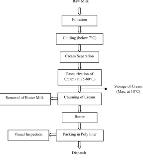
Butter is obtained by churning the cream in a continuously butter making machine forming a compact mass of fat. This system consists of six principal subsystems namely, filter, chiller, separator, pasteurizer, churner and packing. All the units are subject to major failures except filter and packing units, which seldom fail. Hence these have not been considered for analysis. Fig. 1 gives us the flow chart of butter making process.
2.1 System description
2.1.1 Filter subsystem, meant for filtering out any physical impurities in the milk. The accepted milk is weighed and unloaded in the dump tank and filtered. Such milk is then stored in silos through the previously cleaned, sterilized/steamed pipe lines. This system rarely fails.
2.1.2 Chiller subsystem (A): Filtered milk is chilled through a chiller ensuring the temperature not exceeding 7°C. It consists of two units in perfect switch over mode. If one unit fails, the other unit works. Failure of both units results in major failure of the system.
2.1.3 Separator subsystem (B): Cream separation is planned after ensuring sufficient quantity of raw milk for operation of at least 5-6 hours. Like Chiller subsystem, it also contains one main unit and a standby unit. Standby unit comes into operation only when main unit fails. Major failure occurs only when both units fail.
2.1.4 Pasteurizer subsystem (C): In this subsystem, cream is heated upto 80°C with no holding time. Its purpose is to destroy any pathogenic and undesirable bacteria/organisms and deactivate the enzymes present in the milk. Its failure causes the complete failure of the system.
units in parallel. Failure of any one unit reduces the capacity of the system. Failure of both units causes major failure of the system.
2.1.6 Packing subsystem: The butter coming out of the butter making machine is directly packed in poly liner and corrugated boxes. The boxes are weighed and sealed. This system rarely fails.
2.2 Notations
A, B, C, D indicate that the respective subsystems are working at full capacity
a, b, c, d indicate that the respective subsystems are in failed state
As, Bs indicate that one respective subsystem has failed
D' indicate that the respective subsystem is working at reduced
capacity
( = 1 4) indicate the failure rates of subsystems A, B, C and D respectively
( = 1 4) indicate the repair rates of subsystems A, B, C and D respectively
( ) denotes the probability that at time‘t’, all the units are working
( , ) denotes the probability that at time‘t’, the system is in state i and
having an elapsed repair time x
2.3 Assumptions
Present analysis is based on following assumptions:
(i) Failure and repair rates are constant and independent of each other and their unit is taken as per day.
(ii) In case of assessment of availability using SVT, repair rates are considered variable and failure rates as constant.
(iii) Performance wise, a repaired unit is as good as new.
(iv) Service and repair/ maintenance and replacement facilities are available. Fig. 1. Schematic diagram of butter production system
Dispatch
Storage of Cream (Max. at 10°C) Filtration
Removal of Butter Milk
Chilling (below 7°C)
Cream Separation
Pasteurization of Cream (at 75-80°C)
Churning of Cream
Butter Raw Milk
(v) There are no simultaneous failures.
(vi) System may work at reduced capacity.
3. Mathematical Formulation of the System
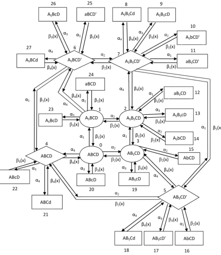
To determine the reliability of the butter production system, we develop Chapman-Kolmogorov differential eqs. by applying SVT. Probability considerations, using mnemonic rule, give us the following set of differential eqs. associated with the transition diagram (Fig. 2) of the system at time (t+∆t):
Fig. 2. Transition diagram of butter production system α1
16 ASBSCd
ASBSCD'
ASBScD
ASbCD'
aBSCD' ASBCD'
aBCD' ASBcD
ASBCd
ASBSCD
aBSCD
ASBScD
ASbCD
ABSCD
AbCD
ABSCD' ABScD
ABCD ASBCD aBCD
ASBcD
ABcD ABCD
ABcD
ABCd
ABSCd ABScD' AbCD
1 0 24 2 3 19 17 18 5 20 21 22
4 14
15 12
13 27
23
26 25 8 9
10
11 6
7
β1(x)
β2(x) β3(x)
β4(x)
α2 α3 α4 α4 α1 α4 α4 α4 α4 α1
β1(x)
α3
β3(x)
α2
β2(x) β4(x)
β1(x)
α2 β2(x) α3
β3(x)
β4(x)
α1
β1(x)
α3
β3(x)
α2 β2(x) α4
α1 β1(x)
α2 β2(x)
α3 β3(x) β
4(x)
α2
β2(x)
α1 β1(x)
β4(x)
α3 β3(x)
α3
β3(x)
β4(x)
α2
β2(x)
β4(x)
α3 β
3(x)
α1 β1(x)
α4
β4(x)
α1 β1(x)
( + ∆ ) = 1 − ∆ − ∆ − ∆ − ∆ ( ) + ( ) ( , ) ∆ + ( ) ( , ) ∆ +
( ) ( , ) ∆ + ( ) ( , ) ∆
( + ∆ ) − ( ) =
− ∆ + ∆ + ∆ + ∆ ( ) + ( ) ( , ) ∆ + ( ) ( , ) ∆ +
( ) ( , ) ∆ + ( ) ( , ) ∆
Dividing both sides by ∆ , we get
( ∆ ) ( )
∆ =
− + + + ( ) + ( ) ( , ) + ( ) ( , ) + ( ) ( , ) +
( ) ( , )
+ ( ) = ( ) (1)
+ + ( ) ( , ) = ( , ) (2)
+ + ( ) ( , ) = ( , ) (3)
+ + ( ) ( , ) = ( , ) (4)
+ + ( ) ( , ) = ( , ) (5)
+ + ( ) ( , ) = ( , ) (6)
+ + ( ) ( , ) = ( , ) (7)
+ + ( ) ( , ) = ( , ) (8)
+ + ( ) ( , ) = 0; = 11,12,24,25
(9)
+ + ( ) ( , ) = 0; = 10,14,15,16
(10)
+ + ( ) ( , ) = 0; = 9,13,17,19,20,22,23,26
(11)
+ + ( ) ( , ) = 0; = 8,18,21,27 (12)
Where,
= ∑
( ) = ∑ + ( )
( ) = ∑ + ( ) + ( )
( ) = ∑ + ( )
( ) = ∑ + ( )
( ) = ∑ + ( ) + ( )
( ) = ∑ + ( ) + ( ) + ( )
( ) = ( ) ( , ) + ( ) ( , ) + ( ) ( , ) + ( ) ( , )
( , ) = ( ) + ( ) ( , ) + ( ) ( , ) + ( ) ( , ) +
( ) ( , )
( , ) = ( ) + ( ) + ( ) ( , ) + ( ) ( , ) + ( ) ( , ) +
( ) ( , )
( , ) = ( ) + ( ) ( , ) + ( ) ( , ) + ( ) ( , ) +
( ) ( , )
( , ) = ( ) + ( ) ( , ) + ( ) ( , ) + ( ) ( , ) +
( ) ( , )
( , ) = ( ) + ( ) + ( ) ( , ) + ( ) ( , ) + ( ) ( , ) +
( ) ( , )
( , ) = ( ) + ( ) + ( ) ( , ) + ( ) ( , ) + ( ) ( , ) +
( ) ( , )
( , ) = ( ) + ( ) + ( ) + ( ) ( , ) + ( ) ( , ) + ( ) ( , ) +
( ) ( , )
Initial Conditions
(0) = 1
( , 0) = 0 ( = 1,2,3 … … … … . .27)
Boundary Conditions (0, ) = ( ) (0, ) = ( , ) + ( , )
(0, ) = ( ) (0, ) = ( )
(0, ) = ( , ) + ( , ) (0, ) = ( , ) + ( , )
(0, ) = ( , ) + ( , ) + ( , ) (0, ) = ( , ) (0, ) = ( , )
(0, ) = ( , ) (0, ) = ( , )
(0, ) = ( , ) (0, ) = ( , )
(0, ) = ( , ) (0, ) = ( , )
(0, ) = ( , ) (0, ) = ( , )
(0, ) = ( , ) (0, ) = ( , )
(0, ) = ( ) (0, ) = ( , )
(0, ) = ( , ) (0, ) = ( , )
(0, ) = ( , ) (0, ) = ( , )
Set of differential eqs. from (1) to (12) along with initial conditions and boundary conditions is called Chapman-Kolmogorov differential difference eqs. Eq. (1) is a linear differential eq. of first order and eqs. (2) to (12) are linear partial differential eqs. of first order (Lagrange's type). All these eqs. have been solved using Lagrange’s method. The probabilities of each state and expression of availability has been derived as follows:
( ) = 1 + ( )
( , ) = ( ) ( , ) ( ) + ( − )
( , ) = ( ) ( , ) ( ) + ( , − ) + ( , − )
( , ) = ( ) ( , ) ( ) + ( − )
( , ) = ( ) ( , ) ( ) + ( − )
( , ) = ( ) ( , ) ( ) + ( , − ) + ( , − )
( , ) = ( ) ( , ) ( ) + ( , − ) + ( , − )
( , ) = ( ) ( , ) ( ) + ( , − ) + ( , − ) + ( , − )
( , ) = ( ) ( , − )
( , ) = ( ) ( , − )
( , ) = ( ) ( , − )
( , ) = ( ) ( , − )
( , ) = ( ) ( , − )
( , ) = ( ) ( , − )
( , ) = ( ) ( , − )
( , ) = ( ) ( , − )
( , ) = ( ) ( , − )
( , ) = ( ) ( , − )
( , ) = ( ) ( , − )
( , ) = ( ) ( , − )
( , ) = ( ) ( − )
( , ) = ( ) ( , − )
( , ) = ( ) ( , − )
( , ) = ( ) ( , − )
( , ) = ( ) ( , − )
( , ) = ( ) ( , − )
( , ) = ( ) ( , − )
Finally, the expression of time dependent availability A(t) is obtained by summation of probabilities of all the working states and reduced capacity states, i.e.
( ) = ( ) + ∑ ( , )
(13) Availability expression of the butter production system as given by eqn. (13) can be solved using constant failure rates and variable repair rates from the concerned plant.
3.1 Availability of the system when failure and repair rates are constant
It is very difficult to solve the problem if either failure rate or repair rate are varied. In order to simplify the problem, failure and repair rates are considered constant. In this case, the system of eqs. (1) to (12) can be represented as follows:
( ) + ∑ = ( ) + ( ) + ( ) + ( ) (14)
( ) + ∑ + = ( ) + ( ) + ( ) + ( ) + ( ) (15)
( ) + ∑ + + = ( ) + ( ) + ( ) + ( ) + ( ) + ( ) (16)
( ) + ∑ + = ( ) + ( ) + ( ) + ( ) + ( ) (17)
( ) + ∑ + = ( ) + ( ) + ( ) + ( ) + ( ) (18)
( ) + ∑ + + = ( ) + ( ) + ( ) + ( ) + ( ) + ( ) (19)
( ) + ∑ + + = ( ) + ( ) + ( ) + ( ) + ( ) + ( ) (20)
( ) + ∑ + + + = ( ) + ( ) + ( ) + ( ) + ( ) + ( ) +
( ) (21)
( ) + = ( ) (22)
= 11, = 7; = 12, = 2; = 24, = 1; = 25, = 6
( ) + = ( ) (23)
= 10, = 7; = 14, = 2; = 15, = 3; = 16, = 5
= 9, = 7; = 13, = 2; = 17, = 5; = 19, = 3; = 20, = 0; = 22, = 4; = 23, = 1; = 26, = 6
( ) + = ( ) (25)
= 8, = 7; = 18, = 5; = 21, = 4; = 27, = 6
Initial Conditions
( ) = 1 = 0
= 0 ≠ 0
To examine the effect of failure and repair rates on the availability in transient state, the system of differential eqs. (14) to (25) with initial conditions has been solved numerically using Runge-Kutta fourth order method. Analysis has been done for a period of 360 days divided over an interval of 30 days and the data has been tabulated in tables 1-8. These tables present the effect of failure and repair rates of various subsystems on the reliability of the system. MTBF, which has been computed using Simpson’s 3/8 rule, with corresponding failure rates, has been given in the last row of each table.
4. Results and Analysis
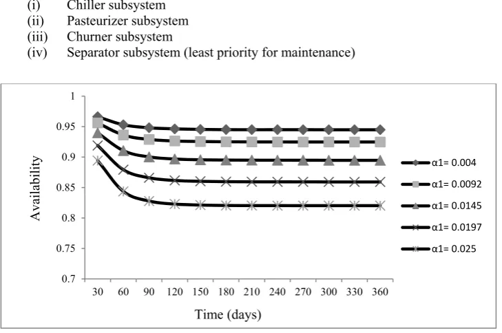
Effect of failure rate of chiller (α1) on system availability
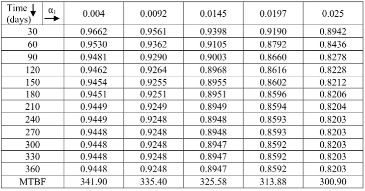
By varying failure rate α1 from 0.004, 0.0092, 0.0145, 0.0197 and 0.025 and keeping α2 = 0.002, α3 = 0.001666, α4 = 0.003333, β1 = 0.05, β2 = 0.03333, β3 = 0.0416 and β4 = 0.03333, the availability of the system has been computed and compiled in Table 1, which shows that there is a decrease in availability upto 12.46 percent. Also availability decreases by upto 7.39 percent with the increase in time from 30 to 360 days. MTBF shows a decline of 41 days with the increase in failure rate from 0.004 to 0.025.
Table 1. Effect of failure rate of chiller (α1) on availability
Time
(days) α1 0.004 0.0092 0.0145 0.0197 0.025
30 0.9662 0.9561 0.9398 0.9190 0.8942
60 0.9530 0.9362 0.9105 0.8792 0.8436
90 0.9481 0.9290 0.9003 0.8660 0.8278
120 0.9462 0.9264 0.8968 0.8616 0.8228
150 0.9454 0.9255 0.8955 0.8602 0.8212
180 0.9451 0.9251 0.8951 0.8596 0.8206
210 0.9449 0.9249 0.8949 0.8594 0.8204
240 0.9449 0.9248 0.8948 0.8593 0.8203
270 0.9448 0.9248 0.8948 0.8593 0.8203
300 0.9448 0.9248 0.8947 0.8592 0.8203
330 0.9448 0.9248 0.8947 0.8592 0.8203
360 0.9448 0.9248 0.8947 0.8592 0.8203
MTBF 341.90 335.40 325.58 313.88 300.90
Effect of failure rate of separator (α2) on system availability
Table 2. Effect of failure rate of separator (α2) on availability
Time
(days) α2 0.002 0.003423 0.004846 0.006269 0.00769
30 0.9662 0.9645 0.9621 0.9590 0.9552
60 0.9530 0.9496 0.9446 0.9383 0.9307
90 0.9481 0.9436 0.9372 0.9291 0.9196
120 0.9462 0.9412 0.9341 0.9252 0.9147
150 0.9454 0.9402 0.9327 0.9234 0.9125
180 0.9451 0.9397 0.9321 0.9226 0.9115
210 0.9449 0.9395 0.9318 0.9222 0.9110
240 0.9449 0.9394 0.9317 0.9220 0.9107
270 0.9448 0.9394 0.9316 0.9219 0.9106
300 0.9448 0.9394 0.9316 0.9219 0.9106
330 0.9448 0.9394 0.9316 0.9219 0.9105
360 0.9448 0.9394 0.9316 0.9219 0.9105
MTBF 341.90 340.25 337.88 334.92 331.44
Effect of failure rate of pasteurizer (α3) on system availability
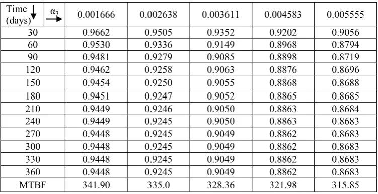
Next, we have studied the effect of failure rate of pasteurizer on the availability of casting system. The results shown in Table 3 indicate that by varying failure rate α3 = 0.001666, 0.002638, 0.003611, 0.004583 and 0.005555 and taking α1 = 0.004, α2 = 0.002, α4 = 0.003333, β1 = 0.05, β2 = 0.03333, β3 = 0.0416 and β4 = 0.03333, the availability decreases by 7.66 percent. It is also observed that there is a decrease of 3.73 percent in availability with the increase in time from 30 to 360 days. In this case, MTBF decreases by 26 days with the increase in failure rate.
Table 3. Effect of failure rate of pasteurizer (α3) on availability
Time
(days) α3 0.001666 0.002638 0.003611 0.004583 0.005555
30 0.9662 0.9505 0.9352 0.9202 0.9056
60 0.9530 0.9336 0.9149 0.8968 0.8794
90 0.9481 0.9279 0.9085 0.8898 0.8719
120 0.9462 0.9258 0.9063 0.8876 0.8696
150 0.9454 0.9250 0.9055 0.8868 0.8688
180 0.9451 0.9247 0.9052 0.8865 0.8685
210 0.9449 0.9246 0.9050 0.8863 0.8684
240 0.9449 0.9245 0.9050 0.8863 0.8683
270 0.9448 0.9245 0.9049 0.8862 0.8683
300 0.9448 0.9245 0.9049 0.8862 0.8683
330 0.9448 0.9245 0.9049 0.8862 0.8683
360 0.9448 0.9245 0.9049 0.8862 0.8683
MTBF 341.90 335.0 328.36 321.98 315.85
Effect of failure rate of churner (α4) on system availability
Table 4. Effect of failure rate of churner (α4) on availability
Time
(days) α4 0.003333 0.005277 0.007222 0.009166 0.011111
30 0.9662 0.9628 0.9580 0.9521 0.9450
60 0.9530 0.9459 0.9364 0.9248 0.9115
90 0.9481 0.9390 0.9269 0.9124 0.8960
120 0.9462 0.9361 0.9227 0.9068 0.8889
150 0.9454 0.9348 0.9208 0.9043 0.8857
180 0.9451 0.9342 0.9200 0.9031 0.8842
210 0.9449 0.9340 0.9196 0.9025 0.8835
240 0.9449 0.9339 0.9194 0.9023 0.8832
270 0.9448 0.9338 0.9193 0.9021 0.8830
300 0.9448 0.9338 0.9192 0.9021 0.8830
330 0.9448 0.9338 0.9192 0.9020 0.8829
360 0.9448 0.9338 0.9192 0.9020 0.8829
MTBF 341.90 338.55 334.10 328.81 322.88
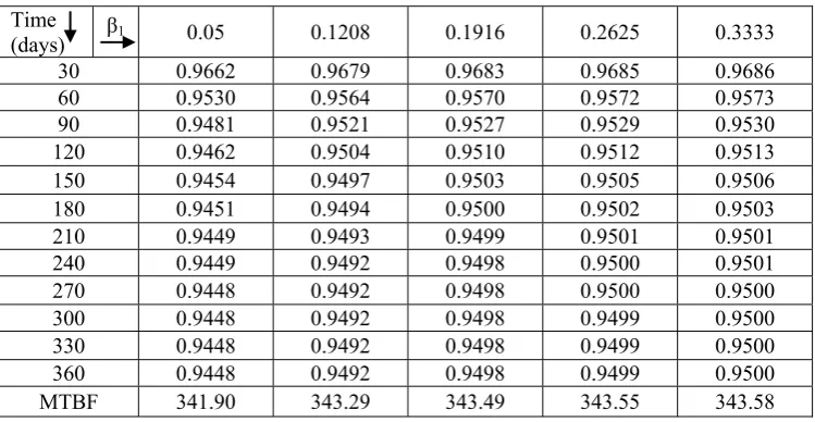
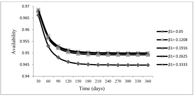
Effect of repair rate of chiller (β1) on system availability
The results presented in Table 5 indicate the availability of the system when repair rate β1 of the chiller subsystem is varied from 0.05 to 0.3333. Taking values of α1 = 0.004, α2 = 0.002, α3 = 0.001666, α4 = 0.003333, β2 = 0.03333, β3 = 0.0416 and β4 = 0.03333, one can see that availability improves upto 0.52 percent. Whereas, there is a decrease of 1.86-2.14 percent in availability as number of days increase from 30 to 360. MTBF increases by around 2 days with the increase in repair rate.
Table 5. Effect of repair rate of chiller (β1) on availability
Time
(days) β1 0.05 0.1208 0.1916 0.2625 0.3333
30 0.9662 0.9679 0.9683 0.9685 0.9686
60 0.9530 0.9564 0.9570 0.9572 0.9573
90 0.9481 0.9521 0.9527 0.9529 0.9530
120 0.9462 0.9504 0.9510 0.9512 0.9513
150 0.9454 0.9497 0.9503 0.9505 0.9506
180 0.9451 0.9494 0.9500 0.9502 0.9503
210 0.9449 0.9493 0.9499 0.9501 0.9501
240 0.9449 0.9492 0.9498 0.9500 0.9501
270 0.9448 0.9492 0.9498 0.9500 0.9500
300 0.9448 0.9492 0.9498 0.9499 0.9500
330 0.9448 0.9492 0.9498 0.9499 0.9500
360 0.9448 0.9492 0.9498 0.9499 0.9500
MTBF 341.90 343.29 343.49 343.55 343.58
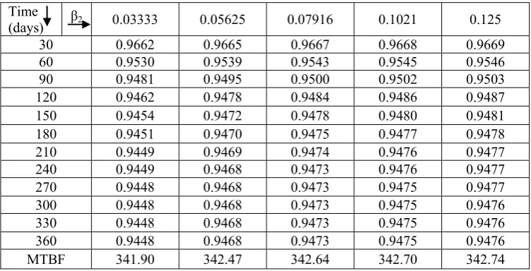
Effect of repair rate of separator (β2) on system availability
Table 6. Effect of repair rate of separator (β2) on availability
Time
(days) β2 0.03333 0.05625 0.07916 0.1021 0.125
30 0.9662 0.9665 0.9667 0.9668 0.9669
60 0.9530 0.9539 0.9543 0.9545 0.9546
90 0.9481 0.9495 0.9500 0.9502 0.9503
120 0.9462 0.9478 0.9484 0.9486 0.9487
150 0.9454 0.9472 0.9478 0.9480 0.9481
180 0.9451 0.9470 0.9475 0.9477 0.9478
210 0.9449 0.9469 0.9474 0.9476 0.9477
240 0.9449 0.9468 0.9473 0.9476 0.9477
270 0.9448 0.9468 0.9473 0.9475 0.9477
300 0.9448 0.9468 0.9473 0.9475 0.9476
330 0.9448 0.9468 0.9473 0.9475 0.9476
360 0.9448 0.9468 0.9473 0.9475 0.9476
MTBF 341.90 342.47 342.64 342.70 342.74
Effect of repair rate of pasteurizer (β3) on system availability
Table 7 shows the effect of improvement of repair rate of pasteurizer on the overall system availability. We see that as β3 increases from 0.0416 to 0.0666 and the value of failure and repair rates of other subsystems are kept at α1 = 0.004, α2 = 0.002, α3 = 0.001666, α4 = 0.003333, β1 = 0.05, β2 = 0.03333 and β4 = 0.03333, availability shows an increase of 1.36 percent. But as the number of days increase from 30 to 360, there is a decrease of around 1.45-2.14 percent in the value of availability. MTBF increases by around 4 days with the increase in repair rate.
Table 7. Effect of repair rate of pasteurizer (β3) on availability
Time
(days) β3 0.0416 0.04792 0.0542 0.0604 0.0666
30 0.9662 0.9681 0.9699 0.9715 0.9729
60 0.9530 0.9566 0.9597 0.9622 0.9644
90 0.9481 0.9524 0.9559 0.9587 0.9610
120 0.9462 0.9508 0.9544 0.9572 0.9596
150 0.9454 0.9501 0.9537 0.9566 0.9589
180 0.9451 0.9498 0.9534 0.9563 0.9586
210 0.9449 0.9496 0.9533 0.9561 0.9585
240 0.9449 0.9496 0.9532 0.9561 0.9584
270 0.9448 0.9495 0.9532 0.9561 0.9584
300 0.9448 0.9495 0.9532 0.9560 0.9584
330 0.9448 0.9495 0.9532 0.9560 0.9584
360 0.9448 0.9495 0.9532 0.9560 0.9584
MTBF 341.90 343.40 344.59 345.52 346.31
Effect of repair rate of churner (β4) on system availability
Table 8. Effect of repair rate of churner (β4) on availability
Time
(days) β4 0.03333 0.07499 0.11666 0.15833 0.2
30 0.9662 0.9674 0.9679 0.9682 0.9683
60 0.9530 0.9564 0.9573 0.9577 0.9578
90 0.9481 0.9530 0.9540 0.9543 0.9545
120 0.9462 0.9519 0.9529 0.9532 0.9534
150 0.9454 0.9515 0.9525 0.9528 0.9530
180 0.9451 0.9514 0.9524 0.9527 0.9528
210 0.9449 0.9513 0.9523 0.9526 0.9528
240 0.9449 0.9513 0.9523 0.9526 0.9528
270 0.9448 0.9513 0.9523 0.9526 0.9528
300 0.9448 0.9513 0.9523 0.9526 0.9528
330 0.9448 0.9513 0.9523 0.9526 0.9528
360 0.9448 0.9513 0.9523 0.9526 0.9528
MTBF 341.90 343.80 344.13 344.24 344.30
5. Conclusion
By comparing the results computed in of Tables 1-8, it reveals that subsystem A (chiller) has maximum impact on the availability as well as on MTBF of the system. This phenomenon has been depicted in the Figs. 3 and 4. Second most important subsystem is C i.e. pasteurizer. However, subsystem B i.e. separator has least impact on the availability and MTBF of the system. Hence, we infer that as far as maintenance planning and scheduling on the basis of failure/repair rates is concerned, the maintenance priority should be given as per the following order:
(i) Chiller subsystem
(ii) Pasteurizer subsystem
(iii) Churner subsystem
(iv) Separator subsystem (least priority for maintenance)
Fig. 3. Effect of failure rate of Chiller on availability 0.7
0.75 0.8 0.85 0.9 0.95 1
30 60 90 120 150 180 210 240 270 300 330 360
α1= 0.004
α1= 0.0092
α1= 0.0145
α1= 0.0197
α1= 0.025
Time (days)
Av
ailab
Fig. 4. Effect of repair rate of Chiller on availability
References
[1] Yang, J; et al. (2008): An N-component series repairable system with repairman doing other work and priority in repair. J Mod Appl Sci, 2(6), pp. 163-168.
[2] Garg, S; Singh, J; Singh, D. V. (2010): Mathematical modelling and performance analysis of combed yarn production system: based on few data, J Appl Math Model, 34(11), pp. 3300-3308.
[3] Gupta, P; Goyal, A. (2010): Availability assessment of a multi-state repairable bubble gum production system, In: Proceedings of IEEE ICIEEM’10. Macao: IEEE, pp. 631-635.
[4] Shakuntla, S; et al. (2011): Reliability analysis of polytube industry using supplementary variable technique, J Appl Math Comput, 218(8), pp. 3981-3992.
[5] Wu, W; et al. (2014): Reliability analysis of a k-out-of-n:G repairable system with single vacation, J Appl Math Model, 38(24), pp. 6075-6097.
[6] Zheng, F; Xu, S; Li, X. (2015): Numerical solution of the steady-state probability and reliability of a repairable system with three unites, J Appl Math Comput, 263, pp. 251-267.
[7] Cekyay, B; Ozekici, S. (2015): Reliability, MTTF and steady-state availability analysis of systems with exponential lifetimes, J Appl Math Model, 39(1), pp. 284-296.
[8] Qamber, I. S. (1999): Reliability study of two engineering models using LU decomposition, J Reliab Eng Syst Safe, 64(3), pp. 359-364.
[9] Garg, S; Singh, J; Singh, D. V. (2010): Availability analysis of crank-case manufacturing in a two-wheeler automobile industry, J Appl Math Model, 34(6), pp. 1672-1683.
[10] Li, L; Yan, H; Wu, X. (2012): Numerical analysis on the reliability of space tracking, telemetering and command system based on the sparse matrix storage schemes, In: Proceedings of ICQR2MSE’12. Chengdu: IEEE, pp. 240-244.
[11] Nugraha, A. S. (2015): The selection of time step in Runge-Kutta fourth order for determine deviation in the weapon arm vehicle, In: proceedings of ICSEEA’14 2: Elsevier, pp. 363-369.
[12] Amann, C; Kadau, K. (2016): Numerically efficient modified Runge-Kutta solver for fatigue crack growth analysis, J Eng Fract Mech, 161, pp. 55-62.
[13] Hussain, K; Ismail, F; Senu, N. (2016): Solving directly special fourth-order ordinary differential equations using Runge-Kutta type method, J Comput Appl Math, 306, pp. 179–199.
0.94 0.945 0.95 0.955 0.96 0.965 0.97
30 60 90 120 150 180 210 240 270 300 330 360
β1= 0.05
β1= 0.1208
β1= 0.1916
β1= 0.2625
β1= 0.3333
Time (days)
Av
ailab