Earth Surf. Dynam., 6, 239–255, 2018 https://doi.org/10.5194/esurf-6-239-2018 © Author(s) 2018. This work is distributed under the Creative Commons Attribution 4.0 License.
Unsupervised detection of salt marsh platforms:
a topographic method
Guillaume C. H. Goodwin1, Simon M. Mudd1, and Fiona J. Clubb1,2 1School of GeoSciences, University of Edinburgh, Edinburgh, UK
2Institute of Earth and Environmental Science, University of Potsdam, Potsdam, Germany
Correspondence:Guillaume C. H. Goodwin ([email protected])
Received: 11 October 2017 – Discussion started: 1 November 2017 Revised: 31 January 2018 – Accepted: 20 February 2018 – Published: 28 March 2018
1 Introduction
Salt marshes are highly dynamic ecosystems, sequestering on average 210 g CO2m−2yr−1 through plant growth and decay (Chmura et al., 2003) and capturing additional inor-ganic sediment when they are submerged (Nardin and Ed-monds, 2014). This productivity has allowed salt marshes to match historic sea level rise (Kirwan and Temmerman, 2009) and laterally expand when sediment inputs were sufficient (Kirwan et al., 2011). It also places them among the most valuable ecosystems in the world (Costanza et al., 1997), and they provide diverse ecosystem services such as flood attenu-ation (Möller and Spencer, 2002; Shepard et al., 2011), blue carbon sequestration (Chmura et al., 2003; Coverdale et al., 2014), and contaminant capture (Nelson and Zavaleta, 2012). Their economic value combined with their alarming retreat (Day et al., 2000; Duarte et al., 2008; Kirwan and Megoni-gal, 2013) makes monitoring the evolution of salt marshes crucial for developing management strategies that maintain the health of these ecosystems.
The most closely monitored properties of salt marsh ecosystems are ecological assemblages and elevation, as they are both essential to understanding ecogeomorphic processes (Reed and Cahoon, 1992). For instance, elevation determines flooding frequency and therefore influences pioneer vege-tation encroachment (Hu et al., 2015), which in turn af-fects vertical accretion through inorganic sediment capture (Pennings et al., 2005; Mudd et al., 2004, 2010). Individual plants also react to elevation by modifying their root-to-shoot length ratios, generating feedbacks between organic material build-up and sediment capture (Mudd et al., 2009). The vari-able intensity of these ecogeomorphic feedbacks envari-ables salt marshes to accrete in response to variations in sea level, thus maintaining their place in the tidal frame (Kirwan and Tem-merman, 2009; Crosby et al., 2016).
The objective detection and analysis of vegetation patterns is a mature field, with habitat mapping commonly undertaken through the analysis of spectral properties such as the nor-malised difference vegetation index (NDVI; Jucke van Bei-jma, 2015). NDVI mapping is now developed to the extent that it requires only a minimum of ground truthing to deter-mine the presence and type of vegetation (Hladik and Alber, 2014). This index has been shown to consistently differenti-ate vegetdifferenti-ated areas from tidal flats (Tuxen et al., 2008) and flooded channels from dry land despite the sensitivity of clas-sification algorithms (Belluco et al., 2006; Wang et al., 2007). However, spectral data sources do not provide the to-pographic information necessary to fully understand mor-phodynamic processes: although digital elevation models (DEMs) have been successfully generated from habitat maps in the Venice lagoon (Silvestri et al., 2003), additional in-fluences on halophyte distribution such as groundwater cir-culation (Moffett et al., 2010, 2012) can lead to mismatches between topography and habitats (Hladik et al., 2013). These additional influences on habitat distribution prevent the
reli-able use of spectral data to infer topography. Furthermore, delineating salt marsh platforms exclusively from spectral sources encourages morphological studies to define salt marshes dominantly from an ecological perspective, whereas the physical setting, most notably the elevation within the tidal frame, plays a key role in maintaining ecosystem health (e.g. Morris et al., 2002).
The topographic data necessary to identify marsh plat-forms already exist: the proliferation of freely available high-resolution topographic datasets from lidar or structure from motion (SfM) techniques means that DEMs with a grid cell size below 1 m are increasingly common on salt marshes and offer vertical accuracies below 20 cm even without correcting for vegetation (Sadro et al., 2007; Wang et al., 2009; Chas-sereau et al., 2011). At these resolutions, most scarps and channels are detectable on a DEM, and several automated to-pographic methods already allow the identification of tidal channel networks (Fagherazzi et al., 1999; Liu et al., 2015). However, contrary to spectral datasets, tools designed to ac-curately delineate the extent of salt marshes through means other than manual digitisation are lacking.
In this study, we propose an unsupervised method to to-pographically differentiate marsh platforms from tidal flats, which we refer to as Topographic Identification of Platforms (TIP). The TIP method aims to reproducibly and accurately delineate marsh platforms using only a DEM as input, while also reducing identification costs and enabling systematic to-pographic analyses of multiple salt marshes.
G. C. H. Goodwin et al.: Unsupervised detection of salt marsh platforms: a topographic method 241 2 Methodology
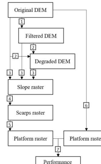
The TIP method automatically detects scarps and platforms of salt marsh systems from a DEM with no manual calibra-tion requirements. Its general process is described in Fig. 1 and includes the possibility of filtering (step 1) and degrading (step 2) the DEM; the effects of both treatments are examined in the discussion. A slope raster is then generated by fitting a polynomial surface to topographic data and taking the deriva-tive of this surface (Hurst et al., 2012; Grieve et al., 2016) (step 3). Steps 4 and 5 are novel algorithms developed in this study to isolate scarps and platforms. The results of the iso-lation process are compared to manually generated platforms (step 6) to generate a comparison map (step 7).
2.1 Test sites
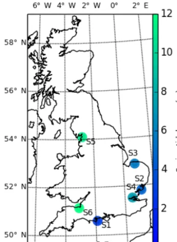
We test the TIP method on six sites in England, se-lected for the availability of airborne lidar data in the form of gridded 1 m resolution rasters, provided by the UK Environment Agency (http://environment.data.gov.uk/ ds/survey/), and for the diversity of their morphologies and tidal ranges. Dataset metadata are available freely on the Environment Agency website (https://data.gov.uk/dataset/ lidar-composite-dtm-1m1). For each site, marsh platforms were digitised on an unfiltered and non-degraded DEM at a scale of 1:500, using the open-source software QGIS (step 6 in Fig. 1). Source data were flown in 2012 for all sites, un-less noted otherwise. The locations of the selected sites are shown in Fig. 2.
Shell Bay, Dorset (S1), is a shallow bay with a spring tidal range of 2.4 m, located in Poole Harbour, a limited entrance bay (sensu Allen, 2000) protected from strong waves. The marshes in Shell Bay display jagged outlines, indicative of low wave and tidal current stress (Leonardi and Fagherazzi, 2014). The Stour Estuary marshes (S2) 6 km upstream of the mesotidal Stour mouth are subject to a spring tidal range of 3.8 m and fluviotidal currents due to their estuarine fringing position (sensu Allen, 2000) and therefore display more lin-ear boundaries. The Stiffkey marshes (S3) are back-barrier marshes (Allen, 2000), which experience a 4.7 m spring tidal range and display signs of erosion and accretion. These re-cent perturbations to the marsh surface provide an interest-ing challenge for topographic detection of marsh extents. The macrotidal Medway estuary marshes (S4, spring tidal range of 6.4 m) were chosen due to the presence of numerous chan-nels in the tidal flats. In order to test the ability of our method in regions with extreme tidal ranges, we also analysed two megatidal sites: Jenny Brown’s Point marshes (S5, spring tidal range of 9.2 m) and the Parrett estuary (S6, spring tidal range of 11.8 m), where sand dunes, different elevations in-side the tidal flats, fallen blocks, and sunken platforms will test the limits of the method’s ability to correctly delineate marshes in these environments.
Figure 1. Flow chart showing the overall structure of the TIP method and its validation. Each object (rectangle) is obtained by im-plementing a routine (square), numbered as follows: 1. implemen-tation of a Wiener filter (optional); 2. subsampling by average value (optional); 3. calculation of slope by fitting a second-order polyno-mial surface; 4. scarp identification by routing; 5. platform identi-fication by dispersion; 6. manual digitisation of a marsh platform; 7. comparison of the objectively detected platform to the manually digitised platform.
2.2 Preprocessing topographic data
Figure 2.This map shows the six sites selected from the lidar col-lection of the UK environment agency, coloured by spring tidal range. The sites are numbered as follows: S1: Shell Bay, Dorset; S2: Stour Estuary, Suffolk; S3: Stiffkey, Norfolk; S4: Medway Estu-ary, Kent; S5: Jenny Brown’s Point, Lancashire; S6: Parrett EstuEstu-ary, Somerset.
vegetation cover in the DEM (Hladik and Alber, 2012; Wang et al., 2009; Sadro et al., 2007; Chassereau et al., 2011; Mon-tané and Torres, 2006), we chose not to apply these correc-tions as we wanted to ensure that the TIP method can be ap-plied without information on the vegetation assemblages at a given site.
2.3 Scarp routing
Tidal flats and salt marshes occur mostly on low energy coasts (Allen, 2000), characterised by low local relief and slopes. They therefore display similar local slope values, and this parameter alone is insufficient to differentiate between tidal flats and marsh platforms. Likewise, although marsh platforms are locally higher than tidal flats and channels, this may not be the case for complex depositional environments (e.g. marshes sheltered by a sand spit), where long-shore declivity may cause portions of the tidal flats to be higher than distant emergent platforms. Therefore, elevation alone, though it may be used to visually identify salt marsh plat-forms, is insufficient for objective platform detection. We ad-dress this problem by investigating transition features such as channel banks and erosion scarps, which are outliers in both slope and elevation rasters. These features are commonly de-fined by steep local slopes, particularly in mature and erod-ing systems (Defina et al., 2007; Marani et al., 2013). Fur-thermore, scarps connect marsh platforms to tidal flats and
therefore represent a distinct break in elevation between the two. In this study, we focus on the identification of scarps and steep channel banks as a precursor to the detection of platforms, referred to as step 4 in Fig. 1.
To reduce computational costs, we delineate an initial search space to initiate the detection of scarps by isolating steep areas of the landscape, weighted by their elevation. We first calculate the relief of each pixel,Ri:
Ri=zi−zmin, (1)
wherezi (dimension L) is the elevation of the pixel andzmin (L) is the minimum elevation in the DEM. We then divide this relief by the maximum relief in the DEM to get a dimen-sionless relief at each pixel,Ri∗:
Ri∗= Ri
zmax−zmin
. (2)
A similar procedure is followed for slope, where Rs (di-mensionless) is determined by the slope at a pixel,Si minus the minimum slopeSmin:
Rsi =Si−Smin, (3)
and the dimensionless version is calculated as
Rs∗i = Rsi
Smax−Smin
. (4)
We then multiply these two metrics at each pixel to create the dimensionless parameterPi∗at each pixel:
Pi∗=R∗iRs∗i. (5)
This dimensionless product is useful for highlighting steep areas at high elevations (Fig. 3): the higher the value ofPi∗, the steeper and higher the pixel.Pi∗could vary between 0 and 1, where a value of 0 would mean that a pixel was at both the lowest elevation and gradient in the DEM, and vice versa for a value of 1.
We use the properties of the probability distribution func-tion (pdf) ofP∗ to define the first search space, which we call Ss∗. With the exception of macrotidal sites S5 and S6,
G. C. H. Goodwin et al.: Unsupervised detection of salt marsh platforms: a topographic method 243
Figure 3.(a1–6)Frequency distribution ofP∗for sites S1–6. The greyed portion of the plot represents pixels that are not included in the initial search space Ss∗;(b)raster representation ofP∗for site S1: Shell Bay. Values ofP∗underP∗th use the topographic colour scheme, while values aboveP∗th use the copper colour scheme and are included in Ss∗.
this study, we optimise the threshold value Spthresh to im-prove the classification of each site, as described in the results section. The first search space, Ss∗, is defined as those pixels whereP∗> P∗th, as shown in Fig. 3b. The search space Ss∗ is also schematically represented as grey cells in Fig. 4a (step 4.1)
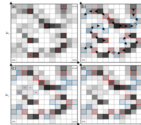
We then define a square kernelK3of three cells in width around each cell in Ss∗. If more than one cell of K3 is in-cluded in Ss∗, the cell containing the local slope maximum inK3is flagged as a first-order scarp cell Sc1. If one given K3 already contains an Sc1 cell that is not the central cell, the central cell will be flagged as an Sc1if, and only if, it is the next local maximum inK3. This results in patchwork of first-order scarp cells (step 4.2 in Fig. 4a).
For each first-order scarp cell (Sc1), we then flag two second-order cells (Sc2) as neighbouring cells with the next steepest slopes contained in the search space and not in con-tact with each other (red outlines in Fig. 4b). If two Sc1 cells are adjacent, only the cell with the higher slope will be flagged as a Sc2cell (step 4.3 in Fig. 4b). This generates a patchwork of first-order cells (black outlines Fig. 4b) flanked
Figure 4. Schematic example of the scarp detection process through maximum slope routing. Panel(a)shows two steps. Step 4.1: determination of the search space Ss∗ (greyed cells, darker with arbitrary slope). Step 4.2: determination of local maxima Sc1 (black outlines with a plus sign).(b) Step 4.3: determination of Sc2cells (red outlines). Step 4.4: determination of Scncells,n >2 (blue outlines).(c)Step 4.5: elimination of cells where max(ZK9)< 0.85×q75(dashed outlines with a minus sign).(d)Step 4.6: elim-ination of isolated cells (dashed outlines with a minus sign). The arrows represent the progressive selection of scarp cells.
by one or two second-order cells (red outlines in Fig. 4b). Starting from the second-order cells (Sc2), we prolong the scarps by finding the cell with the steepest slope that is not adjacent to another identified scarp cell of two lesser orders, within aK3kernel centred on the previously identified cell. For example, on the third iteration, Sc3cells are identified in aK3kernel centred on a Sc2cell and must not be adjacent to an Sc1cell. Generally, Scncells are identified in aK3kernel centred on a Scn−1cell and must not be adjacent to an Scn−2 cell. This routing procedure is applied in all kernels contain-ing no more than two scarp cells and repeated until no cells fit the conditions or the ordernis equal to 100 (blue outlines, step 4.4 in Fig. 4b).
Fig. 4c), where ZKthreshis a parameter which we optimise be-low. EachK9kernel containing less than eight flagged cells is then discarded from the ensemble of scarps; after this pro-cedure finishes, we are left with the final ensemble of scarps (step 4.6 in Fig. 4d).
2.4 Platform identification
We identify marsh platforms based on the final ensemble of scarps (step 5 in Fig. 1). The final ensemble of scarps be-comes a new search space (Ss2). We then create a square ker-nel three cells in width (K3) around each cell in this new search space. Using this kernel we identify first-order plat-form cells, Pc1, which are defined as all cells withinK3that have higher elevation values than the central cell of the ker-nel (i.e. those that are higher in elevation than the cells in the final scarp ensemble). We do this because platform cells are located at higher elevations than the scarp cells separat-ing them from tidal flats. We use a kernel rather than a simple blanket elevation threshold over the entire DEM because lon-gitudinal elevation variations may cause some tidal flat cells to be higher than scarp cells. Each Pc1cell that is not adja-cent to at least two other Pc1cells is considered a product of isolated situations and eliminated from the ensemble of platform cells.
Following this initial selection of platform cells, we pro-ceed to iteratively fill the platforms. At this point, the initial ensemble of platform cells, Pc1, is clustered around the final ensemble of scarps since we have only used a three-pixel-wide kernel centred on scarp cells to create the ensemble of Pc1cells. We then iterate using a filling algorithm. The first iteration uses the cells Pc1, the second Pc2, and so on. In each iteration of Pcncells, new cells are identified using two ker-nels, one being larger than the other. First, we define a local elevation condition using an 11-pixel-wide kernel K11: we find the maximum elevation in this kernel and then subtract 20 cm to define the minimum local elevation for a platform pixel. The 20 cm leeway is applied to account for local el-evation variations on the platforms. The algorithm will not identify separate platforms separated by scarps less than this elevation threshold, so on microtidal marshes this threshold can be lowered. We address this limitation in the discussion and Appendix. The threshold is necessary to prevent the al-gorithm from excluding pools and slight depressions in the platform surface.
We then use a three-pixel-wide kernel (K3) withinK11to identify any cells in the next iterations’ platform ensemble (Pcn+1). These cells must meet two conditions: (i) they are higher than the local elevation threshold identified with the 11-pixel kernel, and (ii) their distance to the nearest cell in the final scarp ensemble is greater than their distance to plat-form cells from previous iterations. The first condition is sim-ply to ensure the platform is indeed a low-relief surface, and the second is to ensure the iterative process fills the platform away from the scarps. The second condition is also necessary
to ensure the platform filling process does not cross scarps. This iterative process is repeated untilnreaches an arbitrary value of 100, found to be sufficient to fill the entirety of the platform surface area for our sites.
This process results in platform surfaces that are spatially continuous, but in some instances sections of the tidal flat with relatively high elevations may also have been identi-fied as marsh platforms. These areas are lower than marsh platforms by the height of the scarp separating them. We fil-ter these cells by using the elevation properties of the en-tire DEM. A number of authors have shown that there is a gap in the probability distribution of elevations in intertidal landscapes that separates the majority of tidal flats from the majority of marsh platforms in microtidal environments (e.g. Fagherazzi et al., 2006; Defina et al., 2007; Carniello et al., 2009). Such a separation, demonstrated by the decrease in probability between the grey and blue surfaces in Fig. 5, is also observed in our meso- and macrotidal sites, including megatidal environments such as the Parrett estuary (Fig. 9). We search for this separation using the probability distribu-tion of elevadistribu-tion, pdf(z), of all cells Pcn, divided in 100 el-evation bins. We determine that the most frequent elel-evation bin,zmax(pdf(z)), is the most likely to contain cells correctly assigned to the platform ensemble, as the relief of marsh plat-forms is lower than that of tidal flats. Therefore, only eleva-tions lower thanzmax(pdf(z)) may contain cells misidentified as marsh platforms.
We then must identify which cells from the population of cells lower than zmax(pdf(z)) form part of the platform, and which do not. To do this, we truncate low elevations that have a low probability (red curves in Fig. 5) to remove the long tail of low elevations from our initial platform identification. We take the probability distribution of the elevation of the remaining platform cells and calculate the mean probability pdf (i.e. we average the probability from the 100 bins). We then search forrzthreshconsecutive elevation bins that lie be-low the elevation of the maximum probability elevation that have lower probabilities than this average. The reason we use consecutive bins is that we do not want the minimum eleva-tion to be determined by a single low-probability elevaeleva-tion that has spuriously arisen from the binning process. Once we findrzthreshconsecutive elevation bins meeting these criteria, we remove all cells lower than and including the highest cell that lies within therzthreshconsecutive bins. We optimise the parameterrzthreshbelow.
G. C. H. Goodwin et al.: Unsupervised detection of salt marsh platforms: a topographic method 245
Figure 5.Diagram describing the elimination of the tail of the el-evation probability distribution function for site S1. The grey filled surface is the pdf of elevation for the original DEM. The dark red line is the pdf of elevation of the platform after the dispersion pro-cess. The orange line is the pdf of elevation of the platform after truncation of the tail of the distribution. The blue line is the pdf of elevation of the platform after filling pools and jagged outlines and after the addition of scarps in the platform ensemble. The dark blue line, associated to the blue filled surface, is the pdf of elevation for the final platform, after the tail of its distribution is truncated a sec-ond time. All distributions in this plot are forced to display the same maximum for clarity.
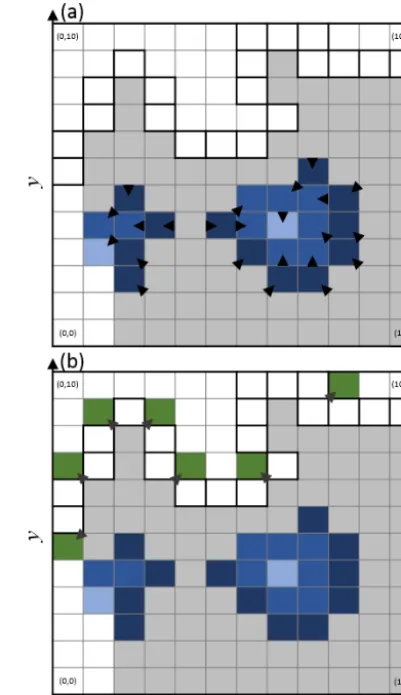
the order 2, we progressively fill pools and jagged borders of the platform (Fig. 6a). Choosing six as the minimal num-ber of platforms cells in each K3 necessary to execute this “reverse filling” procedure, we ensure that no headlands are generated. We then integrate scarp cells that are connected to platform cells into the platform ensemble with an order greater than 100. We then repeat the “reverse filling” pro-cess (Fig. 6b) and execute low-elevation elimination proce-dure (see blue curves in Fig. 5) to obtain the final platform ensemble.
2.5 Performance metrics
In order to evaluate the performance of the TIP method, we compare its outputs to manually digitised platforms for all of our test sites (step 7 in Fig. 1). For each grid cell in the detected (automatically processed) and the reference (man-ually digitised) outputs, we assign the boolean value “true” to the marsh platform and “false” to the tidal flat. The re-sults are classified as follows: true positives correspond to matching true cells in the tested and reference outputs, true negatives to matching false cells, false positives to true cells in the tested output that are false in the reference output, and
Figure 6.Schematic example of the reverse platform filling pro-cess.(a)Step 5.1: filling of empty cells adjacent to Pcncells (grey, dark blue, and blue cells) with an ordern−1 (dark blue, blue, and light blue cells).(b)Step 5.2: filling of empty cells adjacent to Pcn cells (grey cells) with an ordern−1 (green cells) when scarp cells (black outlines) are included in the platform ensemble. The arrows indicate the dispersion pattern.
false negatives to false cells in the tested output that are true in the reference output. The performance of the method is then evaluated using three metrics based on the numbers of true positive (TP), true negative (TN), false positive (FP), and false negative (FN) cells, respectively. The accuracy (Acc) (Fawcett, 2006) describes the likelihood of cells in the tested raster corresponding to the reference raster:
Acc= TP+TN
TP+TN+FP+FN. (6)
the tested raster overestimating the positives compared to the reference:
Pre= TP
TP+FP. (7)
Conversely, the sensitivity, Sen, represents the likelihood of the tested raster missing positives compared to the refer-ence:
Sen= TP
TP+FN. (8)
If the results of the TIP method perfectly matched that of the manual digitisation, all three metrics would have a value of 1.
3 Results
3.1 Parameter optimisation
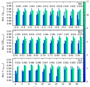
The TIP method contains three user-defined, non-dimensional parameters occurring in sequence during the detection process. The first parameter, Spthresh, de-termines the threshold value P∗th for the high-pass filter leading to the selection of the initial search space, shown in Fig. 3a. The parameter Spthreshinfluences the solution of the equation ddPf∗=Spthresh. The second parameter, ZKthresh, determines the condition on the refinement of existing scarps in the high-pass filter max(ZK9)>ZKthresh×q75, schemat-ically represented in Fig. 4. The third parameter,rzthresh, is used in the platform dispersion process to determine which percentage of the elevation range below pdf is maintained in the platform ensemble. In this study, these parameters were set to maximise the average accuracy (Acc) across test sites (Fig. 7): the optimised values (Spthresh= −2.0, ZKthresh=0.85,rzthresh=8) were used for the subsequent performance analysis. Users may modify these parameters as directed in the code documentation to better fit their study sites.
3.2 Validation and applicability
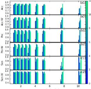
Figure 8 shows the performance of the TIP method for all six sites, discriminating between the use or absence of a Wiener filter and evaluating how the resolution of the topographic data influences the results. We also provide the full perfor-mance metrics in Appendix A (Tables A1 to A6). We find the method’s accuracy to be on average 94.8 % at the data’s native resolution of 1 m, whether we apply a Wiener filter (Fig. 8a2) or not (Fig. 8a1). Degrading the DEM resolution still results in accuracy of above 90 %, although it decreases to around 60 % for microtidal site S1 at a resolution of 3 m. Applying a Wiener filter to the data causes a slight decrease in accuracy and precision (Fig. 8b2), but an increase in sen-sitivity (compare Fig. 8c2 to c1). Examining the results of all
of the metrics shows that resolution degradation up to 3 m, as well as the use of a Wiener filter, primarily causes an increase in false positives and therefore an overestimation in the ex-tent of the marsh platform. For sites S2 to S6, we observe little change in performance metrics with resolution degra-dation up to 3 m.
We suggest that all three performance metrics should be used when optimising the TIP method for a study site, as no combination of two metrics provides comprehensive in-sight into TIP uncertainties. Furthermore, although average accuracies remain above 85 % for resolutions of 4 to 5 m, we recommend caution when using the method at these res-olutions, particularly in micro- to mesotidal settings where features may be smoothed beyond the method’s recognition capacities. Use of the TIP method is not recommended for resolutions coarser than 5 m due to the very low accuracies observed for our test sites, making this method adapted to high-resolution data sources such as airborne lidar or pho-togrammetry.
4 Discussion
4.1 Influence of site morphology on the TIP method
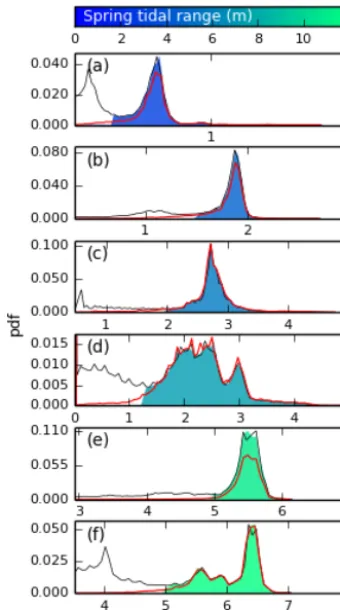
In order to examine the performance of the method in sites with varying morphological characteristics, we compare the probability distribution functions of elevation from the digi-tised platforms to the platforms detected using the TIP method (Fig. 9). Figure 9a–f show that a left-hand tail is present for the digitised platforms, whereas platforms de-tected by TIP show a sharp decrease in the pdf at these eleva-tions: this indicates the presence of more false negatives than false positives at the lowest elevations of the marsh platform. This suggests that the TIP method excludes more features with a low elevation than manual digitisation, which corre-spond to tidal creeks and sunken terraces at the edge of the platform. However, this does not imply that the TIP method cannot identify multiple terraces within a platform, as shown by the multiple local maxima in the detected pdf in Fig. 9d and f.
G. C. H. Goodwin et al.: Unsupervised detection of salt marsh platforms: a topographic method 247
Figure 7.Accuracy charts used to optimise the three user-defined parameters for the six test sites, each site being coloured by spring tidal range, with no filter. Each group of bars represents the accuracy for one parameter value when applied to all the test sites. The mean accuracy appears above each group.(a)Accuracy for the parameter Opt1; the retained value for Opt1 is−2.0.(b)Accuracy for the parameter Opt2; the retained value for Opt2 is 0.85.(c)Accuracy for the parameter Opt3; the retained value for Opt3 is 8.
In our meso- to macrotidal sites S2 to S4 (Fig. 10b–d), the method results in false negatives corresponding to the loca-tion of tidal creeks. These creeks were purposefully included in the marsh platform during the digitisation process but were identified as part of the tidal flat by the TIP method. This re-sult indicates that our method often characterises creek banks as platform scarps due to their morphological similarity.
Other coastal landforms may generate false positives, as seen in Fig. 10c–f. In these cases, the position of the scarp line differs between the digitised and the TIP-detected plat-forms due to elevated portions of the tidal flat being adja-cent to the marsh platform. This suggests that some areas of the tidal flat are topographically closer to the platform than to the rest of the tidal flat and may represent areas likely to be colonised by pioneer vegetation, even though they might not be vegetated at the time of data acquisition. Conversely, sunken platforms or fallen blocks that are not delineated by scarps may generate false negatives, as seen in the central area of Fig. 10e.
Although the TIP method was tested using salt marshes located in England, the scarp and platform association is a common feature to many salt marshes around the world,
making the TIP method applicable over a wide range of geo-graphic areas. Furthermore, the TIP method does not require the precise topography of the platform to function, making it relatively insensitive to unequal removal of vegetation be-tween different DEM sources. The presence of vegetation in-duces positive errors in the DEM, which counter-intuitively may be useful when applying the TIP method, as this artifi-cially increases the platform height and therefore the scarp slope. Examples of sites outside the United Kingdom are in-cluded in Fig. B2 and were selected to demonstrate the ver-satility but also the limits of the TIP method.
4.2 Future developments
Figure 8.Performance of the platform detection method for all sites, coloured according to their spring tidal range;(a1)accuracy of the method when no filter is used;(a2)accuracy of the method when using a Wiener filter;(b1)precision of the method when no filter is used; (b2)precision of the method when using a Wiener filter;(c1)sensitivity of the method when no filter is used;(c2)sensitivity of the method when using a Wiener filter.
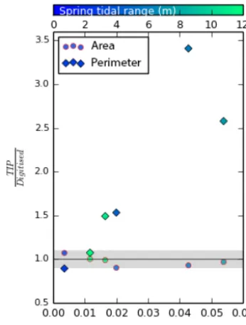
index (DI). In Fig. 11, we examine the capacity of the TIP method to determine the area and perimeter of marsh plat-forms according to their dissection index. We find that for all test sites, TIP-detected area remains within 10 % of the digi-tised area, whereas TIP-detected perimeter increases steadily with dissection index, confirming that the exclusion of tidal creeks by the TIP method is consistently stricter than by digi-tisation. However, neither the TIP method nor manual digiti-sation offers an objective solution to detect tidal creeks. For a comprehensive analysis of marsh platforms, we recommend that objective platform detection be used in conjunction with objective creek detection methods such as those developed by Fagherazzi et al. (1999) and Liu et al. (2015). Further-more, future developments of the TIP method will include an objective creek detection method adapted from these pub-lications, as well as channel network extraction methods de-veloped for fluvial channels by Clubb et al. (2014), to ensure that tidal creeks are detected as separate objects.
The morphological characteristics of prograding marshes are different from those of established platforms: conse-quently, vegetation patches and pioneer zones are not the ob-ject of the TIP method. Specifically, prograding margins and
vegetation patches tend to have a relief and slope that are close to those of the tidal flat, making their outlines invisible to the scarp routing process. The combined absence of scarps and low relief of prograding marshes then interfere with the 20 cm leeway included in the platform filling process and cause an excess of false positives. Users may reduce this lee-way to improve accuracy (see Fig. B2b1), but we discourage the use of the TIP method to identify vegetation patches and prograding margins. However, these dynamic features are the centrepiece of salt marsh development and would benefit from reproducible monitoring methods. Future research may build on the works of Balke et al. (2012) to determine charac-teristic morphologies of prograding marshes, thus providing the necessary groundwork to enable reproducible monitor-ing.
4.3 Potential for monitoring
G. C. H. Goodwin et al.: Unsupervised detection of salt marsh platforms: a topographic method 249
Figure 9.Elevation distribution functions for sites S1 to S6 (panels (a)to(f), respectively). The red line corresponds to the elevation distribution for the reference rasters. The filled area corresponds to the elevation distribution of the automatically processed rasters, coloured according to their spring tidal range. The grey line repre-sents the elevation distribution of the original DEM, with frequency maxima set to match those of the automatically processed rasters so as to nullify the effect of empty cells.
the capacity of the TIP method to monitor temporal change through the example of site S6, which was affected by heavy rainfall in the summer of 2007, resulting in high discharge in rivers such as the Parrett. The 1 m lidar data distributed by the Environment Agency shows that between March and October 2007 the north-eastern corner of site S6 underwent significant erosion. Blue pixels indicating loss of elevation (between March and October) in Fig. 12a bear the character-istic shape of slope failures and intersect the both the auto-matically and manually detected platform outline of March 2007, showing that the October platform outline is further inland.
This retreat of the marsh platform is observed both by the objectively classified (Fig. 12b) and the manually digitised platforms (Fig. 12c). However, whereas the digitisation ef-fort focuses on the large bank failures, the TIP method also detects small changes in the DEM at the platform margin (visible in Fig. 12a and b) and may detect them as changes in marsh platform extent. Consequently, despite a close
corre-Figure 10. Rasters comparing digitised versus extracted marsh platforms superimposed on hillshade data for all six sites after tection with no Wiener filtering. Black areas are outside of the de-tection domain and contain no data. Yellow areas correspond to true positives (TPs) and transparent areas to true negatives (TNs). Red areas correspond to false positives (FPs) and blue areas to false negatives (FNs). Ticks are placed 50 m apart. The sites are num-bered as follows:(a)Shell Bay, Dorset;(b)Stour Estuary, Suffolk; (c)Stiffkey, Norfolk;(d)Medway Estuary, Kent;(e)Jenny Brown’s Point, Lancashire;(f)Parrett Estuary, Somerset.
spondence between TIP-determined marsh outlines and digi-tised outlines (Fig. 12a) near the bank failures, the digidigi-tised volume loss is only 81 % of the objectively detected vol-ume loss. Pioneer zones, characterised by shallow slopes and rapid, uneven elevation changes, are also likely to generate small topographic differences between the DEMs.
5 Conclusions
Figure 11.Ratio of TIP over digitised area (circles, red outlines) and perimeter (diamonds, black outlines) for sites S1 to S6 at the native resolution of 1 m, with no Wiener filtering, as a function of dissection index. Here, dissection index is defined as the ratio of the total length of tidal channels within the digitised marsh platform over the area of the digitised marsh platform and is not bounded by drainage basins. The greyed area corresponds to a 10 % buffer around the line of equationy=1.
analyses and monitoring, particularly for eroding marshes where scarps are clearly defined. Independence from envi-ronmental variables means that our method can be used to complement spectral data for identifying plant types, to bet-ter understand feedbacks between sedimentation, deposition, and biomass. We tested our method on six sites with a wide range of spring tidal ranges and found that tidal range has no significant impact on the detection accuracy. Furthermore, the presence of algae, kelp, or duckweed as well as vary-ing vegetation reflectance properties, which may induce spe-cific calibrations with spectral methods (Morris et al., 2005), do not affect our results (barring mounds of stranded algae large enough to affect topography). Although we did not test the performance of the TIP method on DEM resolutions finer than 1 m, the option of applying a Wiener filter to re-duce DEM noise is available to accommodate DEMs gener-ated from unclassified point clouds, which have higher sur-face roughness. When combined with creek detection meth-ods, we expect the performance of the TIP method to im-prove with fewer false negatives. This would also allow the discrimination of channel evolution within the marsh plat-form and on the tidal flat, allowing us to simultaneously ex-plore the development of marsh platforms and tidal creeks (D’Alpaos et al., 2007, 2010) in sites with strong tidal forc-ing.
Figure 12.(a)Comparison of marsh areas for a portion of S6 be-tween March (green lines) and October (orange lines) 2007, super-imposed on hillshade data of October 2007. Bright lines correspond to the automatically detected marsh boundary, whereas faded lines correspond to digitised marsh boundaries. Green faded lines are mostly covered by bright green lines. Coloured surfaces indicate el-evation gain or loss between March and October 2007.(b)Map of elevation loss and gain associated to marsh platform evolution, ac-cording to the TIP method. Total volume loss is 1188 m3.(c)Map of elevation loss and gain associated to marsh platform evolution, according to manual digitisation. Total volume loss is 966 m3.
G. C. H. Goodwin et al.: Unsupervised detection of salt marsh platforms: a topographic method 251 Appendix A: TIP performance tables
Table A1.Table of accuracy for sites S1 to S6 (columns) with no Wiener filter, for resolutions varying between 1 and 10 m (rows).
Resolution S1 S2 S3 S4 S5 S6
(m)
1.0 0.907 0.940 0.936 0.967 0.963 0.952
1.5 0.876 0.934 0.948 0.926 0.953 0.950
2.0 0.868 0.921 0.950 0.942 0.945 0.919
2.5 0.891 0.926 0.948 0.955 0.942 0.926
3.0 0.646 0.897 0.944 0.954 0.946 0.935
4.0 0.643 0.861 0.932 0.942 0.945 0.909
5.0 0.869 0.872 0.915 0.927 0.941 0.897
7.5 0.778 0.682 0.804 0.806 0.942 0.376
10.0 0.599 0.771 0.786 0.603 0.882 0.376
Table A2.Table of precision for sites S1 to S6 (columns) with no Wiener filter, for resolutions varying between 1 and 10 m (rows).
Resolution S1 S2 S3 S4 S5 S6
(m)
1.0 0.837 0.979 0.985 0.972 0.973 0.916
1.5 0.763 0.970 0.977 0.974 0.953 0.910
2.0 0.753 0.971 0.976 0.967 0.941 0.890
2.5 0.789 0.961 0.976 0.969 0.942 0.889
3.0 0.518 0.959 0.975 0.974 0.943 0.880
4.0 0.513 0.951 0.977 0.968 0.942 0.835
5.0 0.787 0.936 0.989 0.932 0.932 0.896
7.5 0.765 0.908 0.988 0.956 0.949 0.376
10.0 0.475 0.699 0.992 0.000 0.947 0.376
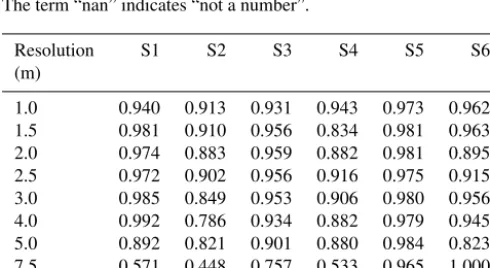
Table A3.Table of sensitivity for sites S1 to S6 (columns) with no Wiener filter, for resolutions varying between 1 and 10 m (rows). The term “nan” indicates “not a number”.
Resolution S1 S2 S3 S4 S5 S6
(m)
1.0 0.940 0.913 0.931 0.943 0.973 0.962
1.5 0.981 0.910 0.956 0.834 0.981 0.963
2.0 0.974 0.883 0.959 0.882 0.981 0.895
2.5 0.972 0.902 0.956 0.916 0.975 0.915
3.0 0.985 0.849 0.953 0.906 0.980 0.956
4.0 0.992 0.786 0.934 0.882 0.979 0.945
5.0 0.892 0.821 0.901 0.880 0.984 0.823
7.5 0.571 0.448 0.757 0.533 0.965 1.000
10.0 0.996 1.000 0.731 nan 0.870 1.000
Table A4.Table of accuracy for sites S1 to S6 (columns) with a Wiener filter, for resolutions varying between 1 and 10 m (rows).
Resolution S1 S2 S3 S4 S5 S6
(m)
1.0 0.900 0.943 0.948 0.961 0.950 0.948
1.5 0.847 0.857 0.948 0.963 0.953 0.950
2.0 0.868 0.854 0.950 0.956 0.945 0.919
2.5 0.890 0.938 0.948 0.964 0.942 0.923
3.0 0.646 0.928 0.947 0.962 0.945 0.935
4.0 0.824 0.832 0.931 0.964 0.945 0.910
5.0 0.717 0.882 0.904 0.961 0.941 0.910
7.5 0.777 0.698 0.854 0.965 0.942 0.376
10.0 0.593 0.771 0.833 0.945 0.870 0.376
Table A5.Table of precision for sites S1 to S6 (columns) with a Wiener filter, for resolutions varying between 1 and 10 m (rows).
Resolution S1 S2 S3 S4 S5 S6
(m)
1.0 0.816 0.978 0.976 0.963 0.948 0.900
1.5 0.716 0.798 0.977 0.961 0.952 0.910
2.0 0.753 0.795 0.976 0.966 0.941 0.989
2.5 0.787 0.774 0.976 0.962 0.942 0.889
3.0 0.518 0.778 0.976 0.951 0.944 0.880
4.0 0.687 0.794 0.979 0.948 0.943 0.841
5.0 0.571 0.846 0.993 0.953 0.932 0.887
7.5 0.757 0.897 0.990 0.962 0.951 0.376
10.0 0.471 0.699 0.995 0.919 0.960 0.376
Table A6.Table of sensitivity for sites S1 to S6 (columns) with a Wiener filter, for resolutions varying between 1 and 10 m (rows).
Resolution S1 S2 S3 S4 S5 S6
(m)
1.0 0.955 0.920 0.957 0.938 0.982 0.971
1.5 0.993 0.997 0.956 0.945 0.981 0.963
2.0 0.974 0.993 0.959 0.920 0.982 0.895
2.5 0.973 0.999 0.956 0.946 0.975 0.909
3.0 0.985 0.961 0.955 0.953 0.977 0.956
4.0 0.976 0.936 0.931 0.961 0.979 0.938
5.0 0.978 0.958 0.883 0.948 0.985 0.823
7.5 0.581 0.489 0.834 0.950 0.964 1.000
Appendix B: Additional test sites and limitations of the TIP method
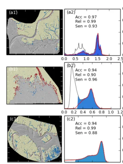
Here, we present three additional sites that demonstrate the capabilities and limits of the TIP method. Sites were selected based on the availability of gridded 1 m DEMs on OpenTo-pography (http://www.opentoOpenTo-pography.org) and on the vari-ety of tidal ranges and climates present: we analyse Morro Bay, CA (A1), Wax Lake Delta, LA (A2), and Plum Island, MA (A3; see Fig. B1). As is common of marshes in the United States, these additional sites have a lower relief than many European marshes, with site A2 displaying a relief of 0.8 m. The performances of the TIP method are recorded in Fig. B2. Optimisation parameters were maintained within the ranges described in Fig. 7.
Site A1, located in the north-east of Morro Bay, shows an extremely close correspondence between the digitised and TIP-detected platforms, with an accuracy of 97 %. It also demonstrates the ability of the TIP method to detect marsh platforms in DEMs where tidal flats exist at higher eleva-tions, as shown by the similar and non-null probability of the TIP-detected and digitised platforms at elevations between 0.3 and 0.9 m (Fig. B2b1). To confirm the observations drawn in the body of the article, site A1 displays an abundance of false negatives within tidal creeks (Fig. B2a1), adding weight to the argument that these features require independent treat-ment.
Site A2 is located on the inside of a marsh island in the rapidly growing Wax Lake Delta. In order to detect the marsh platform with the performance reported in Fig. B2b2, the minimum elevation buffer of 20 cm used in step 5 of Fig. 1 to fill marsh platforms was reduced to 5 cm. This allows the TIP method to function in a site with very low relief and poorly defined scarps. However, we note in Fig. B2b1 that the marginal patches of the marsh are not well identified by the method, as indicated by the relatively large number of false positives on the outline of the marsh. This example therefore demonstrates the difficulties experienced when attempting to detect a prograding marsh by the TIP method. We therefore recommend caution when using the TIP method to monitor prograding marshes, as additional work is needed to fully characterise the topographic signatures of fallen blocks and pioneer zones.
Site A3 is a portion of the well-studied Plum Island, MA. The TIP method yields similar results to site A1, with the notable exception of the bottom right corner of Fig. B2c1. In this area, the marsh platform is heavily dissected by wide, shallow pools and channels, which are commonly excluded from the platform ensemble by the TIP method. Furthermore, the excluded area (containing most false negatives) forms a low, shallow concave surface within the marsh, typically as-sociated with seasonally vegetated areas. These features are morphologically similar to a high tidal flat within the plat-form and are therefore difficult to identify using the TIP method.
Figure B1. This map shows the three additional sites se-lected from the lidar collection of OpenTopography (http://www. opentopography.org), coloured by spring tidal range. The sites are numbered as follows: A1: Morro Bay, California; A2: Wax Lake Delta, Louisiana; A3: Plum Island, Massachusetts.
G. C. H. Goodwin et al.: Unsupervised detection of salt marsh platforms: a topographic method 253 Code and data availability. Our software is freely available for
download on GitHub as part of the Edinburgh Land Sur-face Dynamics Topographic Tools package at https://github.com/ LSDtopotools. The software used in this study is available in this release: https://github.com/LSDtopotools/LSDTopoTools_ MarshPlatform/releases/tag/v0.2 (Goodwin et al., 2017).
Author contributions. GCHG designed the method with contri-butions from other authors. GCHG wrote the code and produced the figures, with support from SMM and FJC in integrating methods with existing channel extraction and topographic processing algo-rithms. GCHG wrote the paper with contributions from other au-thors.
Competing interests. The authors declare that they have no con-flict of interest.
Acknowledgements. Guillaume C. H. Goodwin was supported by a NERC doctoral training partnership grant (NE/L002558/1). Simon M. Mudd was supported by the Leverhulme Foundation (IAF-2014-009). Fiona J. Clubb was supported by NERC grant NE/P012922/1. The authors acknowledge the United Kingdom Environment Agency for the consequent amount of lidar data (point cloud and gridded) made freely available through their website. The authors thank Dimitri Lague for his insightful comments.
Edited by: David Lundbek Egholm Reviewed by: two anonymous referees
References
Allen, J. R. L.: Morphodynamics of Holocene salt marshes: A review sketch from the Atlantic and Southern North Sea coasts of Europe, Quaternary Sci. Rev., 19, 1155–1231, https://doi.org/10.1016/S0277-3791(99)00034-7, 2000. Balke, T., Klaassen, P. C., Garbutt, A., Van der Wal, D., Herman,
P. M. J., and Bouma, T. J.: Conditional outcome of ecosys-tem engineering: A case study on tussocks of the salt marsh pioneer Spartina anglica, Geomorphology, 153–154, 232–238, https://doi.org/10.1016/j.geomorph.2012.03.002, 2012. Balke, T., Herman, P. M. J., and Bouma, T. J.: Critical
tran-sitions in disturbance-driven ecosystems: Identifying Win-dows of Opportunity for recovery, J. Ecol., 102, 700–708, https://doi.org/10.1111/1365-2745.12241, 2014.
Belluco, E., Camuffo, M., Ferrari, S., Modenese, L., Silvestri, S., Marani, A., and Marani, M.: Mapping salt-marsh vegetation by multispectral and hyperspectral remote sensing, Remote Sens. Environ., 105, 54–67, https://doi.org/10.1016/j.rse.2006.06.006, 2006.
Carniello, L., Defina, A., and D’Alpaos, L.: Morphological evo-lution of the Venice lagoon: Evidence from the past and trend for the future, J. Geophys. Res.-Earth, 114, 1–10, https://doi.org/10.1029/2008JF001157, 2009.
Chassereau, J. E., Bell, J. M., and Torres, R.: A comparison of GPS and lidar salt marsh DEMs, Earth Surf. Proc. Land., 36, 1770– 1775, https://doi.org/10.1002/esp.2199, 2011.
Chmura, G. L., Anisfeld, S. C., Cahoon, D. R., and Lynch, J. C.: Global carbon sequestration in tidal, saline wetland soils, Global Biogeochem. Cy., 17, 1111, https://doi.org/10.1029/2002gb001917, 2003.
Clubb, F. J., Mudd, S. M., Milodowski, D. T., Hurst, M. D., and Slater, L. J.: Objective extraction of channel heads fromhigh-resolution topographic data, Water Resour. Res., 50, 4840–4847, https://doi.org/10.1002/2013WR015167, 2014.
Costanza, R., Arge, R., Groot, R. D., Farberk, S., Grasso, M., Han-non, B., Limburg, K., Naeem, S., O’Neill, R. V., Paruelo, J., Raskin, R. G., Suttonkk, P., and van den Belt, M.: The value of the world ’ s ecosystem services and natural capital, Nature, 387, 253–260, https://doi.org/10.1038/387253a0, 1997.
Coverdale, T. C., Brisson, C. P., Young, E. W., Yin, S. F., Donnelly, J. P., and Bertness, M. D.: Indirect human impacts reverse cen-turies of carbon sequestration and salt marsh accretion, PLoS ONE, 9, 1–7, https://doi.org/10.1371/journal.pone.0093296, 2014.
Crosby, S. C., Sax, D. F., Palmer, M. E., Booth, H. S., Deegan, L. A., Bertness, M. D., and Leslie, H. M.: Salt marsh persistence is threatened by predicted sea-level rise, Estuar. Coast. Shelf S., 181, 93–99, https://doi.org/10.1016/j.ecss.2016.08.018, 2016. D’Alpaos, A., Lanzoni, S., Marani, M., Bonometto, A.,
Cec-coni, G., and Rinaldo, A.: Spontaneous tidal network for-mation within a constructed salt marsh: Observations and morphodynamic modelling, Geomorphology, 91, 186–197, https://doi.org/10.1016/j.geomorph.2007.04.013, 2007. D’Alpaos, A., Lanzoni, S., Marani, M., and Rinaldo, A.: On the
tidal prism-channel area relations, J. Geophys. Res.-Earth, 115, 1–13, https://doi.org/10.1029/2008JF001243, 2010.
Day, J. W., Britsch, L. D., Hawes, S. R., Shaffer, G. P., Reed, D. J., Cahoon, D., Britsch, L. D., Reed, D. J., Hawes, S. R., and Ca-hoon, D.: Pattern and process of land loss in the Mississippi Delta: A spatial and temporal analysis of wetland habitat change, Estuaries, 23, 425–438, https://doi.org/10.2307/1353136, 2000. Defina, A., Carniello, L., Fagherazzi, S., and D’Alpaos,
L.: Self-organization of shallow basins in tidal flats and salt marshes, J. Geophys. Res.-Earth, 112, 1–11, https://doi.org/10.1029/2006JF000550, 2007.
Duarte, C. M., Dennison, W. C., Orth, R. J. W., and Car-ruthers, T. J. B.: The charisma of coastal ecosystems: Addressing the imbalance, Estuar. Coast., 31, 233–238, https://doi.org/10.1007/s12237-008-9038-7, 2008.
Fagherazzi, S., Bortoluzzi, A., Dietrich, W. E., Adami, A., Lan-zoni, S., Marani, M., and Rinaldo, A.: Tidal networks 1. Au-tomatic network extraction and preliminary scaling features from digital terrain maps, Water Resour. Res., 35, 3891–3904, https://doi.org/10.1029/1999WR900236, 1999.
Fagherazzi, S., Carniello, L., D’Alpaos, L., and Defina, A.: Crit-ical bifurcation of shallow microtidal landforms in tidal flats and salt marshes, P. Natl. Acad. Sci. USA, 103, 8337–8341, https://doi.org/10.1073/pnas.0508379103, 2006.
Ecolog-ical, geormorphic, and climatic factors, Rev. Geophys., 50, 1–28, https://doi.org/10.1029/2011RG000359, 2012.
Fawcett, T.: An introduction to ROC analysis, Pattern Recogn. Lett., 27, 861–874, https://doi.org/10.1016/j.patrec.2005.10.010, 2006. Feagin, R. A., Martinez, M. L., Mendoza-Gonzalez, G., and Costanza, R.: Salt marsh zonal migration and ecosystem service change in response to global sea level rise: A case study from an urban region, Ecol. Soc., 15, 1–15, 2010.
Goodwin, G. C. H., Mudd, S. M., and Clubb, F. J.: LSDtopo-tools Marsh Platform Identification Tool, Tech. rep., Zenodo, https://doi.org/10.5281/zenodo.1007788, 2017.
Grieve, S. W. D., Mudd, S. M., Milodowski, D. T., Clubb, F. J., and Furbish, D. J.: How does grid-resolution modulate the topographic expression of geomorphic processes?, Earth Surf. Dynam., 4, 627–653, https://doi.org/10.5194/esurf-4-627-2016, 2016.
Hladik, C. and Alber, M.: Accuracy assessment and cor-rection of a LIDAR-derived salt marsh digital ele-vation model, Remote Sens. Environ., 121, 224–235, https://doi.org/10.1016/j.rse.2012.01.018, 2012.
Hladik, C. and Alber, M.: Classification of salt marsh vegetation us-ing edaphic and remote sensus-ing-derived variables, Estuar. Coast. Shelf S., 141, 47–57, https://doi.org/10.1016/j.ecss.2014.01.011, 2014.
Hladik, C., Schalles, J., and Alber, M.: Salt marsh el-evation and habitat mapping using hyperspectral and LIDAR data, Remote Sens. Environ., 139, 318–330, https://doi.org/10.1016/j.rse.2013.08.003, 2013.
Hu, Z., Van Belzen, J., Van Der Wal, D., Balke, T., Wang, Z. B., Stive, M., and Bouma, T. J.: Windows of opportu-nity for salt marsh vegetation establishment on bare tidal flats: The importance of temporal and spatial variability in hydro-dynamic forcing, J. Geophys. Res.-Biogeo., 120, 1450–1469, https://doi.org/10.1002/2014JG002870, 2015.
Hurst, M. D., Mudd, S. M., Walcott, R., Attal, M., and Yoo, K.: Using hilltop curvature to derive the spatial distribu-tion of erosion rates, J. Geophys. Res.-Earth, 117, 1–19, https://doi.org/10.1029/2011JF002057, 2012.
Jucke van Beijma, S.: Remote Sensing – Based Mapping and Mod-elling of Coastal Salt Marsh Habitats Based on Optical , Lidar and Sar Data. Thesis submitted for the degree of Doctor of Phi-losophy at the University of Leicester, PhD thesis, 2015. Kirwan, M. and Temmerman, S.: Coastal marsh response to
his-torical and future sea-level acceleration, Quaternary Sci. Rev., 28, 1801–1808, https://doi.org/10.1016/j.quascirev.2009.02.022, 2009.
Kirwan, M. L. and Megonigal, J. P.: Tidal wetland stability in the face of human impacts and sea-level rise, Nature, 504, 53–60, https://doi.org/10.1038/nature12856, 2013.
Kirwan, M. L., Murray, A. B., Donnelly, J. P., and Corbett, D. R.: Rapid wetland expansion during European settlement and its implication for marsh survival under modern sediment delivery rates, Geology, 39, 507–510, https://doi.org/10.1130/G31789.1, 2011.
Leonardi, N. and Fagherazzi, S.: How waves shape salt marshes, Geology, 42, 887–890, https://doi.org/10.1130/G35751.1, 2014. Liu, Y., Zhou, M., Zhao, S., Zhan, W., Yang, K., and
Li, M.: Automated extraction of tidal creeks from
air-borne laser altimetry data, J. Hydrol., 527, 1006–1020, https://doi.org/10.1016/j.jhydrol.2015.05.058, 2015.
Marani, M., D’Alpaos, A., Lanzoni, S., Carniello, L., and Rinaldo, A.: Biologically-controlled multiple equilibria of tidal landforms and the fate of the Venice lagoon, Geophys. Res. Lett., 34, 1–5, https://doi.org/10.1029/2007GL030178, 2007.
Marani, M., Da Lio, C., and D’Alpaos, A.: Vegetation en-gineers marsh morphology through multiple competing stable states., P. Natl. Acad. Sci. USA, 110, 3259–63, https://doi.org/10.1073/pnas.1218327110, 2013.
Mo, Y., Momen, B., and Kearney, M. S.: Quantify-ing moderate resolution remote sensing phenology of Louisiana coastal marshes, Ecol. Modell., 312, 191–199, https://doi.org/10.1016/j.ecolmodel.2015.05.022, 2015. Moffett, K. B., Robinson, D. A., and Gorelick, S. M.:
Relation-ship of Salt Marsh Vegetation Zonation to Spatial Patterns in Soil Moisture, Salinity, and Topography, Ecosystems, 13, 1287–1302, https://doi.org/10.1007/s10021-010-9385-7, 2010.
Moffett, K. B., Gorelick, S. M., McLaren, R. G., and Sudicky, E. A.: Salt marsh ecohydrological zonation due to heterogeneous vegetation-groundwater-surface water interactions, Water Resour. Res., 48, W02516, https://doi.org/10.1029/2011WR010874, 2012.
Möller, I. and Spencer, T.: Wave dissipation over macro-tidal salt-marshes: Effects of marsh edge typology and vegetation change, J. Coast. Res., 36, 506–521, ISSN: 0749-0208, 2002.
Montané, J. M. and Torres, R.: Accuracy Assessment of Lidar Salt-marsh Topographic Data Using RTK GPS, Photogramm. Eng. Rem. S., 961–967, 2006.
Morris, J. T., Sundareshwar, P. V., Nietch, C. T., Kjerfve, B., and Cahoon, D. R.: Responses of Coastal Wetlands to Rising Sea Level, Ecology, 83, 2869–2877, https://doi.org/10.1890/0012-9658(2002)083[2869:ROCWTR]2.0.CO;2, 2002.
Morris, J. T., Porter, D., Neet, M., Noble, P. A., Schmidt, L., Lapine, L. a., and Jensen, J. R.: Integrating LIDAR elevation data, multi-spectral imagery and neural network modelling for marsh characterization, Int. J. Remote Sens., 26, 5221–5234, https://doi.org/10.1080/01431160500219018, 2005.
Mudd, S. M., Fagherazzi, S., Morris, J. T., and Furbish, D. J.: Flow, sedimentation, and biomass production on a vegetated salt marsh in South Carolina: toward a predictive model of marsh mor-phologic and ecologic evolution, American Geophysical Union, 165–187, https://doi.org/10.1029/CE059p0165, 2004.
Mudd, S. M., Howell, S. M., and Morris, J. T.: Impact of dy-namic feedbacks between sedimentation, sea-level rise, and biomass production on near-surface marsh stratigraphy and carbon accumulation, Estuar. Coast. Shelf S., 82, 377–389, https://doi.org/10.1016/j.ecss.2009.01.028, 2009.
Mudd, S. M., D’Alpaos, A., and Morris, J. T.: How does vege-tation affect sedimenvege-tation on tidal marshes? Investigating par-ticle capture and hydrodynamic controls on biologically me-diated sedimentation, J. Geophys. Res.-Earth, 115, F03029, https://doi.org/10.1029/2009JF001566, 2010.
Nardin, W. and Edmonds, D. A.: Optimum vegetation height and density for inorganic sedimentation in deltaic marshes, Nat. Geosci., 7, 722–726, https://doi.org/10.1038/ngeo2233, 2014. Nelson, J. L. and Zavaleta, E. S.: Salt marsh as a coastal filter
G. C. H. Goodwin et al.: Unsupervised detection of salt marsh platforms: a topographic method 255 in Nitrogen loading and sea-level rise, PLoS ONE, 7, e38558,
https://doi.org/10.1371/journal.pone.0038558, 2012.
Pennings, S. C., Grant, M. B., and Bertness, M. D.: Plant zonation in low-latitude salt marshes: Disentangling the roles of flooding, salinity and competition, J. Ecol., 93, 159–167, https://doi.org/10.1111/j.1365-2745.2004.00959.x, 2005. Reed, D. and Cahoon, D.: The relationship between marsh surface
topography, hydroperiod, and growth of Spartina alterniflora in a deteriorating Louisiana salt marsh, J. Coast. Res., 8, 77–87, 1992.
Robinson, E. A. and Treitel, S.: Principles of Digital Wiener Filtering, Geophys. Prospect., 15, 311–332, https://doi.org/10.1111/j.1365-2478.1967.tb01793.x, 1967. Sadro, S., Gastil-Buhl, M., and Melack, J.: Characterizing
pat-terns of plant distribution in a southern California salt marsh using remotely sensed topographic and hyperspectral data and local tidal fluctuations, Remote Sens. Environ., 110, 226–239, https://doi.org/10.1016/j.rse.2007.02.024, 2007.
Schroder, A., Persson, L., de Roos, A. M., and Lundbery, P.: Direct Experimental Evidence for Alternative Stable States: A Review, Oikos, 110, 3–19, https://doi.org/10.1111/j.0030-1299.2005.13962.x, 2005.
Shepard, C. C., Crain, C. M., and Beck, M. W.: The protective role of coastal marshes: A systematic review and meta-analysis, PLoS ONE, 6, e27374, https://doi.org/10.1371/journal.pone.0027374, 2011.
Silvestri, S., Marani, M., and Marani, A.: Hyperspectral remote sen-ing of salt marsh vegetation, morphology and soil topography, Phys. Chem. Earth, 28, 15–25, https://doi.org/10.1016/S1474-7065(03)00004-4, 2003.
Temmerman, S., Bouma, T. J., Van de Koppel, J., Van der Wal, D., De Vries, M. B., and Herman, P. M. J.: Vegetation causes channel erosion in a tidal landscape, Geology, 35, 631–634, https://doi.org/10.1130/G23502A.1, 2007.
Tuxen, K. A., Schile, L. M., Kelly, M., and Siegel, S. W.: Vegetation colonization in a restoring tidal marsh: A remote sensing approach, Restor. Ecol., 16, 313–323, https://doi.org/10.1111/j.1526-100X.2007.00313.x, 2008. Wang, C., Menenti, M., Stoll, M. P., Belluco, E., and Marani, M.:
Mapping mixed vegetation communities in salt marshes using airborne spectral data, Remote Sens. Environ., 107, 559–570, https://doi.org/10.1016/j.rse.2006.10.007, 2007.
Wang, C., Menenti, M., Stoll, M. P., Feola, A., Belluco, E., and Marani, M.: Separation of ground and low veg-etation signatures in LiDAR measurements of salt-marsh environments, IEEE T. Geosci. Remote, 47, 2014–2023, https://doi.org/10.1109/TGRS.2008.2010490, 2009.