Expression of Maintenance Down Time as
a function of the management mode of the
failure.
L. MEVA’A*
Department of Mechanical Engineering, National Advanced School of Engineering The University of Yaounde I, Cameroon
P.O BOX 8390 Yaounde - Cameroon
R. DANWE
Department of Mechanical Engineering, National Advanced School of Engineering The University of Yaounde I, Cameroon
P.O BOX 8390 Yaounde - Cameroon
T. BEDA College of Technology
The University of Ngaoundere, Cameroon
Abstract:
In production, machine Down Time imputable to maintenance is a permanent preoccupation of services responsible for the proper functioning of production tool. It influences notably the performance of the enterprise and thus, is the main objective of some companies. In this article, we are proposing an expression of the down time of a production chain, resulting from the apparition of a breakdown. The particularity of our approach is to take into account on one part, the hierarchical structure of the maintenance workshop and on the other part, the management mode of the breakdown in the correction process by integrating periodicity in the decision making. Next, we identify the total inactive maintenance time which we wish to reduce following a reduction algorithm.
Keywords: down time; breakdown; periodicity; algorithm; inactive time
1. Introduction
The worry of personnel in a maintenance workshop is to avoid breakdown in order to guarantee a 100% availability of the machines. Given that this objective is difficult to attain, different maintenance personnel have come up with various actions in order to reduce down time. This is done by identifying precisely the different task by level of intervention in the correction process of the breakdown and measuring the duration of these tasks. Quantitative and qualitative study of these different stages further permits us to work on reducing the times considered to be compressible.
Our work is based on observation of the functioning of certain maintenance workshops, notably those of small manufacturing enterprises. In effect, we notice the existence of a periodicity in the dynamic of treatment of some breakdowns of which the gravity slightly influenced the daily performance.
In our article, we precise particular hypotheses on which our work is based. The most significant is the hierarchical structure of the maintenance service which is split into different levels of decision making and the periodicity in decision making by levels.
treatment of the breakdown and the hierarchical organization of the structure having the perturbation. The interest of these works is explained using important stakes in terms of productivity and on the part in terms of the market to which the enterprises make deliveries. We site some examples, those of Ait Kadi [1] on optimization of availability of industrial systems, those of Wang [2] on maintenance model having as goal to maximize the working time of industrial systems. We remark that for many authors, the theme down and up which is the opposite of down is mostly addressed in the framework of research on reliability and maintenance. These two indicators converge to evaluating the availability. Thus, Menye [3] in his work treats down time by optimizing Mean Time To Repair (MTTR). Ireson [4] defined three types of up times which depend on what is included in the definition of mean time to failure (MTTF) and mean down time (MDT). Dhilon [5] as well as Blanchard [6] worked on measurements of the average active time of corrective and preventive maintenance when the system is down.
We will first of all define precisely, the down time, and then express the different hypotheses of our work. Next, we proceed to modeling the down time. We define the notion of inactive time which we identify by an expression. Finally, we propose to reduce these inactive maintenance times using an algorithm.
2. Methodology
2.1 Definition of maintenance down time
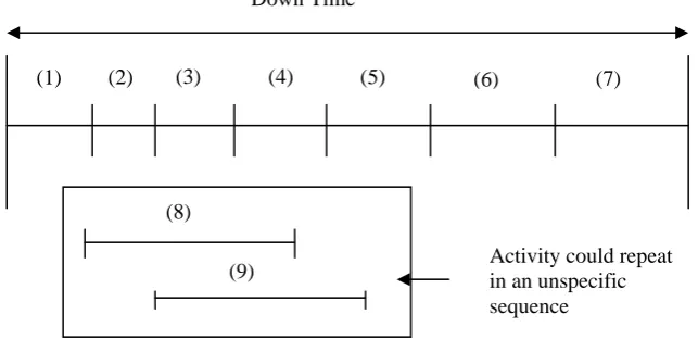
The down time is the period during which the equipment has breakdown [7]. Generally, we avoid all concrete definition, because it’s risky generalizing as a result of parameters which vary with the system and the functioning conditions. We therefore define the down time as a function of the system in question, according to the working conditions and maintenance applicable. Actually, the down time could begin before repairs. And repairs include the control or alignment phases which proceed beyond the duration of unavailability. Therefore, the definition and usage of terms varies depending on what we consider as unavailability or maintenance resources. The significance of terms equally varies depending on whether a system is considered to be, a redundant entity or a replaceable module. Figure 1 shows us the different elements that constitute the period during which the system is down and the repair time.
Fig. 1. Element constituting the down time
Realization time (1): it’s the time that elapses before the failure is noticed.
Access time (2): it’s the time interval between which the failure is noticed and a failure report is posted on the bill board. Taking measurements mark the start of the repairs.
Diagnostic time (3): it’s the detection time of the failure; it includes adjusting the test equipment, executing tests, interpretation of the data collected, verification of the results and choice of corrective measures.
Time to order for spare parts (4): the spare parts are of diverse origins; <tool box> of technicians, recovering identical redundant parts in other areas of the system.
( (
Activity could repeat in an unspecific sequence Down Time
(1) (2) (3) (4) (5) (6) (7)
(8)
Replacement time (5): it is the time needed to remove the damaged part and replace it with the spare part. This time depends mainly on the limitations made between diagnoses and direct replacement as well as the characteristics of the mechanical conception.
Check time (6): it is the time necessary to verify if the failure (breakdown) has been repaired and if the system is operational.
Alignment time (7): introduction of a new module in the system may need adjustments and fitting. Part or all of the time used for this purpose may not be accountable in the duration for which the system is down (duration of unavailability).
Transportation time (8): it’s the delay incurred as a result of transporting workers, spare parts, equipment used to carry out checks and test and supplementary tools to the area were they are used.
Administrative time (9): it includes the organization put in place by the user of the system; generally, it includes establishing reports which will affect; the length of time for which the system is down, distribution of the tasks, re-allocation of manpower in relation to the different task, allocation of breaks, resolution of disputes, etc..
2.2Hypotheses of the work
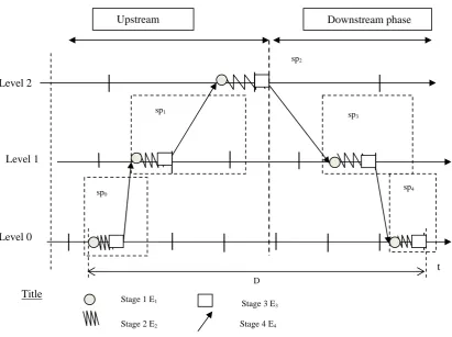
We consider that the maintenance workshop is hierarchical with respect to the organization and it has many levels. Therefore there exist many levels of decision making (Fig. 2). The treatment of a breakdown, which causes a production tool to be down, follows a precise process which is based on the following hypotheses:
- We consider the arrival of the breakdown on a machine to be a disruptive event in the maintenance
workshop.
- We consider the worst case, wherein the event appears at level 0, and is not treated; it creates repercussions right up to the Nth level where it is finally treated. This case, gives the longest down time.
- Propagation of the event: the disturbance appears at a level which cannot treat it; it creates repercussion at a higher level. This repercussion moves from one level to the next until it gets to the level where it is treated. - The functioning is periodic: the repercussion from one level to the next consists of two phases, an upstream
phase which is the ascending phase (from lower to higher levels) and a downstream phase which consist of repercussion of the event at the level where it’s elaborated onto a lower level which has to apply this event. In both phases, the repercussion from one level to the next is done at the end of the period. The conduct in this case is said to be periodic.
- On a given level, the period of the upstream phase is different from the period of the downstream
phase. In effect, once the solution to a breakdown is gotten, the value of the downstream phase is lower than that of the upstream phase.
- Transmission of the event from one level to the next is not instantaneous. There exists a transmission delay upstream and a delay downstream between two consecutive levels. And this delay is not zero.
- On each level, there exist a shift (which could be zero) between the reference date, time origin (t0) and the
Fig. 2. Example of an atelier with 3 levels of making decisions
Our objective presented in the figure 3, is to express the down time of the maintenance workshop having a breakdown, as a function of both the occurrence date of the unwanted event and system parameters, notably, the start dates of the reference periods of the different levels implicated in the treatment.
Fig. 3. Objective of the model
xk(0) : Initialization date of the reference period. u0: Occurrence date of the event.
D: Delay in unavailability (down) of the workshop.
( )
{ }
[
k 0,1,...,N]
k0
0
x
,
u
f
D
=
=We represent a sub process as each passage of a disturbance through a level. Thus, all levels k, except the highest level (k=N), consist of two sub processes spk and sp2N-k which treats the perturbation upstream and
downstream (Fig. 2). The level N at which the disturbance is treated has only one sub process: spN
The process therefore has 2N+1sub processes (0,1,…….,2N). In each sub process i, spi except the last
(i=2N), the event in the upstream phase passes through four successive states, the event in the downstream phase equally passes through four successive states (Table 1). The sub process 2N, sp2N, which is the last, has
just the first three stages. Level 2
S
Stage 2 E2
Stage 3 E3
Stage 4 E4 D
Upstream Downstream phase
Level 1
Level 0
sp0
sp1
sp2
sp3
sp4
Title Stage 1 E1
t
Reaction process Level (N+1)
Entrance Exit
xk(0)k=0,1,…, N
u0
Table1. Different treatment states in a sub process.
State Description Duration
Upstream Phase Downstream Phase
E1 Evaluation of the
gravity
Verification for coherence Ti,1
E2 Preliminary
Traitement
Elaboration of the decision framework Ti,2
E3 Wait for the end of
the period
Wait for the end of the period Ti,3
E4 Transfer to a higher
level
Transfer to a lower level Ti,4
Without much detail about what is happening in the different states, we can simply say that, the state E1 in
the upstream phase determines the mode of periodic or factual treatment, as a function of the gravity.
2.3Model of delay in unavailability
t0 : reference date;
k : level considered;
φ : phase indice;
i : indice of the sub process considered; l : indice of the breakdown state; j : order number of the period;
N : level at which the disturbance is treated; spi : sub process i of the system;
El : state l of the treatment process;
Pkφ : duration of a period at the level k in phase φ ;
jiφ : synchronization period for which the disturbance is treated in spi;
xk(0) : start date of the reference period for the level k; xi0 : arrival date of the disturbance in the sub process spi ;
Ti,,l : duration of state l of spi ;
S : implementation date of the reaction;
T : delay of the system to react to the disturbance; ui : entrance date of the disturbance in the state spi;
xk(j) : finish date of the period j in level k;
xil : finish date from the state E1, of the disturbance of spi;
si : exit date of the disturbance (end of the last stage) from spi;
For a sub process, the treatment sequence is the same. Figure 4 shows the different dates for which the perturbation changes states in the different sub processes.
Fig. 4. Duration and change of state in a sub process spi
All sub processes i (i=0,1,………2N), belong to a phase φ and to a level k which is determine in the following manner:
j xk
(j)
ji ϕ
ui
Ti,4
Ti,2
Ti,1
Pk ϕ
0 1
xk(0)
Ti,3
si xi
0 xi3
t0
≤ = not if 1 N i if 0
ϕ
− ≤ = not if i 2N N i if i kThere exist two distinct dynamics in the treatment process. On one part we have the dynamic of the event (its change of states) which is realized at irregular instances as a function of the duration of the different states which are intrinsic properties of the system with respect to a given disturbance. On the other part, the dynamic of taking decision which is regular, because it’s periodic at each level.
Nevertheless, the two dynamics have to be synchronized in order for the disturbance to pass from state E3 to
state E4 (Fig. 4) in order that decision relative to its transfer can be taken. One of the two dynamic has to adapt
to the other. This is what makes the difference between a periodic and a factual conduct.
In a factual conduct, it’s the dynamic of decision making that has to adapt to that of the disturbance, given that it’s irregular, factual conduct is therefore forced to be irregular. On the contrary, in a periodic conduct, it’s the dynamic of the event that adapts to that of decision making. This is what includes the wait times before treatment of the event.
In reality, the two modes are combined in the description of a mixed conduct. In our case a periodic conduct is needed, but for more critical disturbances, decision is made without waiting for the end of the period.
Passage from one period jφ to the next jφ+1, on a given level k, is executed at the end date of the period k, xk(jφ), which is given either by:
xk(jφ)=Pk+xk(jφ-1)
or:
xk (jφ)=jφPkφ+xk(0)
In periodic conduct, the disturbance is treated in a sub process spi, at the period ji
φ
,, of phase φ of level k (to
which the sub process spi belongs). This is determine in the following manner:
( )
( )
+ + + − = = − + + ∈ ∃ = not if 1 P 0 x T T u E j λP 0 x T T u while IN λ if λ j k k i,2 i,1 i i k k i,2 i,1 i i ϕ ϕ ϕ ϕE represents the real part of x
The dates for the disturbance to change states (transfer from the state El to the state El+1), for each of the 4
states of the sub process spi, xil are given by:
{ }
( )
= = ∈ ∀ + = 3 l j x x 1,2,4 l T x x i k i 3 l i, i 1 -l i l ϕFor i=3, the equation which we have, marks synchronization between the two dynamics. It permits us to determine the date for which transfer decision is taken for treatment of the disturbance. This date coincide with the finish date of the synchronization period jiφ, of the sub process spi.
Entrance ui and exit si from spi in the upstream phase of the periodic process are such that:
=
=
i 4 i i 0 ix
s
x
u
We then obtain:
From above, the exit date is therefore:
Si=xk(0)+jiφPkφ+Ti,4
This result is valid for all sub processes i except for the last sub process i=2N, for which the state E4 does not
exist, consequently T2N,4=0. We have:
S2N=x2N(0)+j2N1P0
The treatment process of a disturbance consist of N+1 levels and 2N+1 sub processes. The disturbance passes through all the sub processes.
The entrance date of the event into a sub process is equal to the exit date of the previous sub process. Entrance data:
=
∀k 0,1,...,N )
0 ( x
u
k
0
Parameters:
{
}
= ∈
∀
= =
∀
exist not does which ) T except ( 0,1,...2N i
et 1,2,4 l
T
0,1 et
N 0,1,..., k
P
2N,4 l
i,
k
ϕ
ϕ
Calculate
For i=0,1,…,2N-1 and φ=0,1
=
+
+
=
+1 i i
i,4 k i k i
s
u
T
P
j
)
0
(
x
s
ϕ ϕFor i=2N
S2N=x0(0)+j2NφP0
The down time represents the time between the occurrence and the end of execution of the reaction to the event. That is the actual action of repairs which corresponds to end of our replacement time. With respect to our model, the difference between the exit date of an event from the process of the reaction (exit date of the last sub process sp2N ) and the occurrence date of the event at the first level 0. This is written either as:
0 2N
u
S
D
=
−
or:
(
)
00 1 2N 0
u
P
j
(0)
x
D
=
+
−
Here we have an expression for the delay in availability as a function of system parameters.
2.4 Minimizing inactive times
At each phase φ and at each level k of making decisions, the stage E3 in the upstream phase and in the
downstream phase represents wait for the end of the period. Accumulation of the wait times for these different stages which we are proposing to minimize constitutes a delay in the treatment process.
+ + =
= = = = 2N 0 i 1 -2N 0 i i,4 2 1 l l i, 2N 0 ii,3 T T
T D
Which is of the form: (a)+(b)
or:
=
= 2N 0 i i,3T
)
a
(
And
+
=
= = = 1 -2N 0 l i,4 2N 0 i 2 1 l l i,T
T
)
b
(
This expression shows that the down time is composed of: - Part (a), which constitutes the inactive times
- Part (b), which are times characteristic to the process and hence are incompressible.
In approaching this expression of unavailability with that obtained previously, the inactive time is written as:
+ =
= = = = 2N 0 i 1 -2N 0 i i,4 2 1 l l i, 2N 0 ii,3 D- T T
T or:
( )
+
+
−
=
= = = = 2N 0 i 1 -2N 0 i i,4 2 1 l l i, 0 0 1 0 1 2N 2N 0 ii,3
j
P
-
u
x
(0)
T
T
T
In this equation, only j2Nl varies as a function of the start dates of the reference period of the levels. All the
other terms are constant, for a given system and for a given disruptive event.
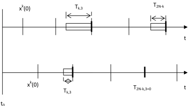
After reducing the down time, it’s imperative to reduce the inactive times, Tk,3 and T2N-k,3 (duration of the
stage E3, o f the two sub processes upstream and downstream appearing at phases 0 and 1 and at level k) by
adjusting the start date of the reference period of the level, xk(0), in a way to eliminate one of the two inactive times (Fig. 5).
Fig. 5. Minimizing inactive times
Tk,3 T2N-k
xk(0)
xk(0)
Tk,3 T2N-k,3=0
t
t
Adjusting on a level is done as follows:
If min(Tk,3 , T2N-k,3) ≤ xk(0), then
xk(0)=xk(0) – min(Tk,3 , T2N-k,3)
if not
xk(0)=Pk0 + [xk(0) - min(Tk,3 , T2N-k,3)]
The result is the elimination of the smaller of the inactive times. We obtain a new start date of the reference period and a new inactive time which is weaker.
For the entire treatment process, we apply successively the same principle to all the levels of the process, starting with the lowest of preference. The algorithm below enables this calculation to be done:
xk(0)=0
∀
φ =0,1 ;∀
k=0,1 ;…,N for k ranging from 0 to N, do :if min(Tk,3 , T2N-k,3)=0, then
k=k+1
if not, if min(Tk,3 , T2N-k,3) ≤ xk(0)
xk(0)= xk(0) - min(Tk,3 , T2N-k,3)
if not
xk(0)=Pk0 + [xk(0) - min(Tk,3 , T2N-k,3)]
end if k=k+1
end if
end
3 Practical example
3.1 Presentation
Considering the example of a maintenance workshop, wherein a breakdown results which needs a spare part. If the worker who is operating on the machine does not have this spare part, he has to address it to the head of the workshop who will address it to the person in charge of the ware house (fore man) who looks for a solution.
The data for the example are as follows:
- time unit is the minute
- the reference date is taken to be some minute which is considered as the time origin. - Occurrence date of the reference minute is: u0=3mn.
- The periods of the levels are: P00=7mn, P10=4mn, P20=2mn, P11 =1mn and P01 =3mn.
- We initialize the reference period of all the levels to the reference date t0=0. That is:
x1(0)=x2(0)=x3(0)=0.
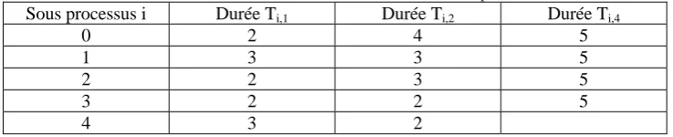
The duration dates for the different stages of each sub process are given in the table 2:
Table 2. Duration of the states of the different sub processes
Sous processus i Durée Ti,1 Durée Ti,2 Durée Ti,4
0 2 4 5 1 3 3 5 2 2 3 5 3 2 2 5 4 3 2
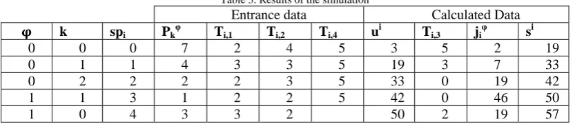
3.2 Results and comments
Table 3. Results of the simulation
Entrance data Calculated Data
k spi Pkφ Ti,1 Ti,2 Ti,4 ui Ti,3 jiφ si
0 0 0 7 2 4 5 3 5 2 19
0 1 1 4 3 3 5 19 3 7 33
0 2 2 2 2 3 5 33 0 19 42
1 1 3 1 2 2 5 42 0 46 50
1 0 4 3 3 2 50 2 19 57
Exit date of the event is si=57mn Duration T=of unavailability is D=54mn The total wait time is 10mn
Next we apply the algorithm to reduce the inactive times on the different levels.
We obtain the following results for each level:
For the level 0, sub processes sp0 and sp4
None of the inactive times is zero, we proceed to the adjustment. The smallest inactive time is T4,3=2mn in
sp0. It is bigger than x0(0)=0. The new value of x0(0) is:
x0(0)=P0+[x0(0)-min(T0,3,T4,3)]=7+(0-2)=5
We have the following results:
Data Parameters Results
u0 x0(0) x1(0) x2(0) T0,3 T1,3 T2,3 T3,3 T4,3 s D Inactive
2 5 0 0 3 1 0 0 0 51 48 4
For the level 1, sub processes sp1 and sp3
The inactive time for sp3 is already zero (T3,3=0), no need to adjust the start date of the reference period for
this level. We maintain x1(0)=0. The result is the same as before.
We have the following results:
Data Parameters Results
u0 x0(0) x1(0) x2(0) T0,3 T1,3 T2,3 T3,3 T4,3 s D Inactive
2 5 0 0 3 1 0 0 0 51 48 4
For level 2, sub process sp2
We do not proceed to any adjustment. The results remain the same.
At the exit from level 2, we obtain an inactive time o f 4min in total which was 10min initially. Converting this to the time unit of the example which is the minute, the reduction of 6min obtained on delay in unavailability which is reduced to 48mins is important.
We think that on the other part that the inactive time of 4mins at the end of the period is incompressible to the extent where, after the principle of the method, one of the two inactive times at a level is zero.
4 Conclusion
We have in this article established a relationship which gives us the down time of a hierarchical maintenance workshop, in a periodic conduct following a breakdown in the system. The delay is expressed as the time between the occurrence of the breakdown and the execution of the reaction. And relation is a function of system characteristics only. We also saw that, delay in unavailability is composed of two parts, one which is incompressible and the other which is the inactive times.
References
[1] Ait-Kadi, D. (1993). Availability optimization for randomly failing equipments: Advanced in Factory of the Future, CIM and Robotics, Elsevier, Manufacturing Research and Technology, 16, p. 333-342.
[2] Wang, H. (2002). A survey of Maintenance Policies of Deteriorating Systems. European Journal of Operational Research, 139: 460-489.
[3] Menye, J;B. (2009). Validation de la maintenabilité et de la disponibilité en conception d’un système multi-composant, Thèse de doctorat, Université de Laval, Université de Strasbourg.
[4] Ireson, W ; Coombs, C.F. ; Moss, R.Y. (1995). Handbook of Reliability Engineering and Management, 2nd Edition McGraw-Hill Companies ISBN 0-07-012750-6.
[5] Dhillon, B.S. (2002). Engineering Maintenance: A modern approach, CRC Press, ISBN 1658716-142-7.
[6] [6] Blanchard, B.S; Fabrycky, W.J. (2005). Systems Engineering and Analysis, 4th Edition, Prentice-Hall International Series in Industrial Systems.