Herrmann Crime Sci (2015) 4:33
RESEARCH
The dynamics of robbery and violence
hot spots
Christopher R. Herrmann
*Abstract
This paper examines how hot spots shift by hour of day and day of week. Hot spot analysis is more likely to have a substantial impact on crime patterns if spatiotemporal shifts are incorporated into the crime analysis process. Even in some of the highest crime neighborhoods in Bronx County (NY), not all micro-level geographies (e.g. street seg-ments and property lots) contain substantial (if any) amounts of crime over the 5-year study period. Moreover, while there are 168 h in a week, even the hottest hot spots do not contain crime 24 h a day, 7 days a week, and 52 weeks a year. Hot spots shift by both space and time and it is important to illustrate these dual shifts when researching and analyzing different levels of geographies and/or hot spots. Spatiotemporal crime analyses are appearing much more frequently in our academic literature in recent years and have become a principal contributor to the progression of routine activities, crime pattern theory, place-management and situational crime prevention. In addition, spatiotem-poral hot spots provide important subject and opportunity context and can help answer some of the questions about what specific types of crime opportunities are available inside of hot spots based on land-use and people’s movement patterns. When studying geographical hot spots, it becomes important to measure and illustrate the inter-related temporal shifts within each of the specific hot spots (i.e. not all hot spots are the same) that are generated. Similarly, when studying temporal hot spots, it is important to measure and illustrate the interrelated spatial shifts within each of the temporal frame(s) that are examined. Examples of space–time and time–space hot spot analysis are provided using violent crime data from the New York City Police Department. Key findings of this research include significant shifting of hot spots from weekday to weekend and afternoon to evening, as well as decisive spatiotempo-ral pattern variations between school-day robberies vs. non-school day robberies.
Keywords: Robbery, Violence, Crime analysis, Spatiotemporal, Routine activities, Hot spots
© 2015 Herrmann. This article is distributed under the terms of the Creative Commons Attribution 4.0 International License (http://creativecommons.org/licenses/by/4.0/), which permits unrestricted use, distribution, and reproduction in any medium, provided you give appropriate credit to the original author(s) and the source, provide a link to the Creative Commons license, and indicate if changes were made.
Background
The crime science and crime analysis communities have become proficient in creating, tracking, and handling hot spots of crime (Chainey and Ratcliffe 2005). Current research (Weisburd et al. 2012; Groff et al. 2010; Ber-nasco and Block 2011; Brantingham et al. 2009; Weisburd et al. 2009) indicates that as crime scientists drill down into the micro-levels of geography (e.g., streets, tax lots, buildings), crime hot spots start to form new shapes (e.g. lines, points, building outlines), sizes, and spatiotemporal patterns.
By developing a more comprehensive understanding of the spatial and temporal variations within violent crime
hot spots at the micro-level, crime prevention and crime control specialists can have a greater impact on appre-hending criminals, police resource allocation and plan-ning, crime modeling and forecasting, and evaluation of crime prevention and crime control programs (Boba 2001; Townsley et al. 2003; Ratcliffe 2004; Johnson et al. 2007). In our continuing state of shrinking government operating budgets, crime scientists and crime analysts need to consider the interrelatedness of spatial and tem-poral shifts in crime patterns when creating, tracking, and handling crime hot spots.
Many studies indicate that crimes are clustered at the neighborhood level, but the entire neighborhood is rarely (if ever) criminogenic and only specific parts of neighbor-hoods contain high concentrations of crime (Taylor 1997; Fagan and Davies 2000; Groff et al. 2010). Prior studies
Open Access
incorrectly assume that the relationships between crime, population, land-use, and business establishment types are both homogenous and spatially stationary (Shaw and McKay 1969; Bursik and Grasmick 1993; Sampson et al. 1997; Morenoff and Sampson 1997). Even at the neigh-borhood level, crime is highly clustered and the highest crime neighborhoods have significant percentages of low or zero crime streets within the neighborhood(s).
A substantial body of research has identified that a small percentage of crime locations (i.e. hot spots) con-tain a significant percentage of crime (Sherman et al. 1989; Block and Block 1995; Eck and Weisburd 1995; Brantingham and Brantingham 1999). One of the cur-rent trends in environmental criminology and crime analysis is the study of crime at more ‘micro’ level places (i.e., buildings, properties, block faces, street segments), a geographic scale/level well below the neighborhood level. Part of this concept of micro-level analysis is known as the 80/20 rule or Pareto’s Principle (Eck et al. 2007; Weis-burd et al. 2012), and reigns true not only in crime pre-vention and crime control, but other areas of the criminal justice field as well [this concept has also been branded as the ‘law of crime concentrations’ by Weisburd et al. (2012)].
The 80/20 rule suggests that by targeting or focusing on the highest 20 % of crime hot spots can have a dra-matic influence on the majority (approximately 80 %) of total crime in the study area. According to the 80/20 rule, the net impact of crime prevention and crime control strategies targeting the 20 % would be much higher than attempting to target an entire neighborhood (or whatever the larger study area is that is being examined).
Environmental criminologists using Pareto’s 80/20 rule have pointed out that not all parks are full of drug users/dealers (Wilcox et al. 2004; Eck et al. 2007; Groff and McCord 2012), not all high schools have high rates of delinquency (Wikstrom et al. 2012; Glover 2002; LaGrange 1999), not all bars contain high rates of assault (Ratcliffe 2012; Newton and Hirschfield 2009; Eck et al. 2007; Gorman et al. 2001), and not all parking lots have high rates of auto theft (Rengert 1997; Clarke and Gold-stein 2003). In fact, even ‘high crime’ neighborhoods con-tain hot spots (high density crime areas) and cold spots (zero/low crime areas), high crime streets and zero/low crime streets, and both ‘good’ (i.e. crime protectors) and ‘bad’ (i.e. crime generators) streets and businesses.
Violent crime (i.e., murder, rape, robbery, assault, and shootings) has declined 73 % in the Bronx since 1990 (NYPD Compstat 2010). In his book, Zimring (2011) suggests that the historic crime drop in New York City is a result of better policing (i.e. CompStat, crime analy-sis, hot spot policing, zero tolerance, stop and frisk) and community crime interventions (including ‘gun buyback’
and drug violence reduction programs). Shifting hot-spots research hopes to advance these trends of increas-ing success for law enforcement crime control strategies, advancement of current environmental criminology theories, and expansion upon existing crime preven-tion frameworks. Integrapreven-tion of theory and new analyses at micro-levels (e.g. street segments and risky facilities) will help crime scientists, police departments, and policy makers better understand the spatial and temporal pro-cesses in the ‘magma’ that fuels today’s crime hot spots.
Data and methodology
The objective of shifting hot spots research is to explore, measure, and illustrate the various spatiotemporal shifts that occur within and between violent crime hot spots. Specifically, this research focuses on spatiotemporal crime shifts within violent crime ‘hot spots’ in the Bronx. The Bronx was selected because it contains a higher per capita violent crime rate (crimes per 1000 residents), as well as a higher crime density (crimes per square mile), compared to the other four counties that comprise the City of New York. While much of the spatiotemporal variation(s) or hot spot ‘shiftiness’ occurs as a result of routine activities and land-use heterogeneity-very few hot spots (if any) appear to be both spatially and tempo-rally stationary.
The research area and data for this study are comprised of various Geographic Information Systems (GIS) data-sets for Bronx County, including violent crime datadata-sets (2006–2010) from the New York City Police Department. The Bronx is geographically organized into 38 neighbor-hoods (note, 36 of the 38 neighborneighbor-hoods are ‘residential’, the other two are categorized as parks/open space and industrial), 12 Police Precincts, 355 Census Tracts, 987 Census Block Groups, 10,781 street segments, 89,211 tax/property lots, and 101,307 buildings (NYC Depart-ment of City Planning 2010; NYPD 2010; NYC Depart-ment of Finance 2010; NYC City Department of Buildings 2010). The Bronx is 42 square miles in area, which makes it 14 % of New York City’s total geographical land area (NYC Department of City Planning 2010). According to the US Census (2000), the population of the Bronx is 1,332,650 which comprises 17 % of the total New York City population.
randomly selected, 90 % of the time they would be of a different race or ethnicity (Newsweek 2009).
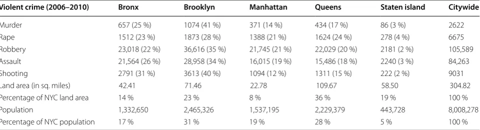
As Table 1 indicates, the Bronx contains a dispropor-tionate amount of violent crime when considering its size (14 % of NYC’s total land area) and population (17 % of NYC’s total population). With the exception of Brooklyn murder and shootings, the Bronx has a much higher dis-proportionate rate of violent crime per capita than all of the other boroughs of New York City. NYPD crime data is geocoded to property lots or intersections, which can then be aggregated up to street segments based on a very accurate, but rather complex, composite address geoloca-tors developed and maintained by the NYC Department of City Planning and the NYC Department of Informa-tion Technology and TelecommunicaInforma-tions.
Research questions
The methods set forth below are designed to address the following research questions.
• How do violent crime hot spots shift from weekday to weekend?
• How do violent crime hot spots shift from daytime to evening/nighttime?
• Are there temporal shifts within and/or between vio-lent crime hot spots?
Hot spots can be calculated many different ways, includ-ing Nearest Neighbor Hierarchical clusters, Getis-Ord Gi* statistics, Kernel Density Estimations, Standard Devia-tion Ellipses, K-Means Clustering, and Local Moran’s I statistics. While any geographic cluster of crime can typi-cally be referred to as a hot spot, not all hot spots are cre-ated equal. It should be noted that none of these hot spot methods take temporal trends into consideration, which is an important function of crime analysis (for more on space–time clustering methods, see Kulldorff 2001).
For this paper, the analysis of violent crime data will include hot spot analysis using the nearest neighbor-hood hierarchical (Nnh) clustering methodology. Nnh hot spots were selected because they generate a specific type of hot spot map which clearly illustrates defined areal boundaries that contain specified concentrations of crime within a specified geographic region, over a spe-cific period of time (Sherman and Weisburd 1995; Mitch-ell 2005).
The nearest neighbor hierarchical clustering (Nnh) routine (in CrimeStat) is simple to understand, runs very quickly on most computers, and is one of the cus-tomary hot spot methodologies for identifying groups or clusters of incidents that are spatially ‘near’ to one another (Harries 1999; Eck et al. 2005; Chainey and Rat-cliffe 2005). The Nnh hot spot routine assembles crimes (points) together based on a pre-defined search criterion (typically, the minimum number of points over a speci-fied geographical area). The clustering routine is then repeated until either all points are grouped into a single cluster or the clustering criterion fails.
The CrimeStat Nnh routine provides the option to clus-ter crimes (points) based on a random or fixed thresh-old search distance and compares this threshthresh-old search distance to the respective distances for all other points within the study area. Only those crimes (points) that are closer to one or more other crimes (points) than the specified threshold distance are selected for clustering. In the crime analysis field, the Nnh routine is commonly used to find the highest concentrations (e.g. robberies per half mile, shootings per kilometer) of crime events over a specified geographic area. Levine (1999) advises that higher frequency crimes (e.g. assault, robbery, auto theft) usually have a much lower threshold distance when compared to lower frequency crimes (e.g. murder, rape, arson) which contain higher threshold distances. Crime clusters can be calculated as convex hulls or ellipses and
Table 1 Violent crime, land area, population, and the percentages for each of the 5 boroughs of New York City by County, for 2006–2010
Source: NYPD Compstat; NYPD Office of Management, Analysis, and Planning; 2012 Census 2000
Violent crime (2006–2010) Bronx Brooklyn Manhattan Queens Staten island Citywide
Murder 657 (25 %) 1074 (41 %) 371 (14 %) 434 (17 %) 86 (3 %) 2622
Rape 1512 (23 %) 1873 (28 %) 1388 (21 %) 1624 (24 %) 278 (4 %) 6675
Robbery 23,018 (22 %) 36,616 (35 %) 21,745 (21 %) 22,029 (20 %) 2181 (2 %) 105,589
Assault 21,564 (26 %) 28,958 (34 %) 16,015 (19 %) 15,486 (18 %) 2240 (3 %) 84,263
Shooting 2791 (31 %) 3613 (40 %) 1094 (12 %) 1311 (15 %) 222 (2 %) 9031
Land area (in sq. miles) 42.41 71.46 22.78 109.67 58.50 304.82
Percentage of NYC land area 14 % 23 % 8 % 36 % 19 % 100 %
Population 1,332,650 2,465,326 1,537,195 2,229,379 443,728 8,008,278
a resulting shapefile can be exported from within the Crimestat software. The primary difference between convex hull and ellipse boundaries are that convex hull boundaries incorporate all of the points within the geo-graphical boundary whereas standard deviational ellipses are a spatial statistical summary and may not incorporate all of the actual points included in the Nnh cluster. In practice, the convex hull selection is ideal when defining hot spot boundaries, while the standard deviational ellip-ses provide an excellent analysis including the direction-ality of the hot spot(s).
As a result of the availability, popularity, comprehen-sive instruction manual, price, and speed of the soft-ware program CrimeStat, the Nnh clustering method has become one of the more popular tools for calculat-ing crime clusters (and crime densities) within the crime science and crime analysis community. However, one of the significant shortcomings of this hot spot method is that Nnh clustering does not take temporal values into its clustering calculation (Chainey and Ratcliffe 2005). While the Nnh clustering analysis provides an excellent clustering technique, it does not provide crime scientists with a statistical test of clustering significance (i.e. Getis-Ord Gi* statistic).
Additionally, there is another free software package that takes temporal values into spatial clustering analysis (SatScan), however this software package is much more complex to learn and is not as widely used in the field of crime analysis (for more on SaTScan, see http://www. satscan.org).
Space–time hot spots vs. time–space hot spots There are two relatively easy processes to construct, examine, and geovisualize the temporal aspects of Nnh hot spots. The first, is a ‘space–time’ analysis, where crime scientists conduct routine spatial hot spot analy-sis and then ascertain the temporal patterns within each of the hot spots. By querying, clipping, and exporting the crime data within each of the spatial hot spots that are generated (import into SPSS or Excel, for example), researchers can detect temporal patterns that are signifi-cant to each spatial hot spot. The results of the tempo-ral analysis after the initial spatial hot spot analysis can further assist crime scientists and analysts in determin-ing what types of targets/victims are present at these hot spots and more importantly, how these targets/vic-tims vary over different time periods (hour of day, day of week, month of year, etc.). In addition, temporal analy-sis can help delineate different types/groups of offenders that may be operating at these locations, as well as expose various offender techniques/modus operandi.
The other way to construct, examine, and geovisualize hot spots is to begin by conducting a temporal analysis
first, before constructing the spatial Nnh hot spots. By defining and analyzing the temporal trend(s) first, crime scientists can identify temporal patterns within the data and then query, clip, and geovisualize these temporal ‘slices’ or aggregates of time data into different hot spot analyses based upon the temporal aspect(s) of interest (e.g. specific days of week, hours of day, weekday vs. weekend). By conducting the temporal analysis before the spatial hot spot analysis, researchers can determine the temporal stability (or variance) of crime patterns and decide more appropriate prevention and control responses according to the temporal (and spatial) clustering.
Temporal trends are becoming increasingly relevant, since this type of data/information provides a much needed crime opportunity context for crime places where crime prevention and control programs are needed, as well as a more structured way of understanding the rou-tine activity patterns of people’s movements based on land-use and business establishment types within micro-level geographies. There are many times where crime pat-terns correlate more with a temporal routine activities trend, as opposed to the spatial clustering relationships that are normally examined and geovisualized without any further temporal analysis (Felson and Boba 2009; Lersch and Hart 2011).
Results and discussion
This section presents the primary findings of the research, as well a dialogue of the results.
Day of week shifts
Much of the impetus for this time–space research pro-cess began with the following day of week and time of day temporal trend analysis (see Figs. 1, 2). For the day of week charts, the days of the week are on the bottom (x-axis) and range from Monday to Sunday and the fre-quency of crime is located on the left (y-axis).
As you can see from Fig. 1, the violent crimes of murder (blue line), shootings (red line), and assaults (yellow line) all follow a very similar day of week pat-tern—smaller numbers of crime on weekdays and then a noticeable shift increase on Friday, Saturday, and Sunday (weekends).
Time of day shifts
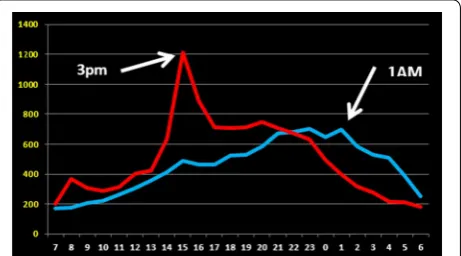
For the time of day figures (Figs. 3, 4), the hour of day is at the bottom (x-axis, ranges from 7 am on the left to 6 am on the right) and the frequency of crime is on the left side (y-axis).
As you can see in Fig. 3, there is a noticeable increas-ing hour of day trend in murder (blue line) and shootincreas-ings (yellow line), which begins around 12 pm/noon and esca-lates until 12 am/midnight, after which, there is a notice-able decline in crime until it levels out around 6 am.
Figure 4 shows that the assault (red line) hour of day trend is very similar to the murder (blue line) and shoot-ing (yellow line) hour of day trends, which increases throughout the daytime, peaks at midnight, and then declines very sharply until it levels out around 6 am. Rob-bery (green line), on the other hand, has a completely different and very abnormal hour of day trend, which steadily increases from 10 am until its highest peak
at 3 pm. Then there is a noticeable shift/decline from 3 pm until 5 pm, after which it slowly increases again until 11 pm, after which it declines sharply and levels off around 6 am.
Further analysis of the NYPD robbery reports indi-cated two very opposing crime patterns (offenders/vic-tims and targets/places). It became evident after reading thru the narratives of many crime reports that the 3 pm robbery spike was largely a result of school-age offend-ers, school-age victims, not surprisingly, near schools and subway stations, on ‘school-days’, and the primary targets were small electronics (e.g. cell phones, tablets, iPods and headsets). The other interesting peak that was noted was a more traditional 12 am/midnight–1 am peak (mostly on weekends). This weekend-nighttime trend mirrored the other traditional violent crime temporal trends noted previously, with the exception that these hot spots were also connected to subway stations (see Fig. 5 below). The nighttime-weekend robbery hot spots also varied sig-nificantly from the daytime-weekday pattern offenders/ victims and targets/places. The nighttime-weekend rob-bery offenders were late teens—early 30’s, the victims were late teens—early 40’s, and the targets were wallets/ purses, jewelry, and cell phones.
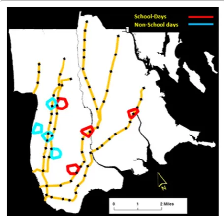
As a result of the relationship between offenders, vic-tims, and places/schools for the 3 pm crime peak, a time–space analysis was conducted and the total robbery points data was disaggregated, by school weeks (weeks when public schools are in session vs. weeks when public schools are not in session), over the 5-year study period. The results indicate a much different ‘temporal-spatial landscape’, than the original (aggregated) robbery map (Fig. 6). The resulting robbery data was then ‘queried and clipped’ into two peak time periods, the 3 pm school-day robbery points and the 1 am non-school day robbery
Fig. 1 Day of week trend for murder. Day of week trend for shootings. Day of week trend for assaults
points, and then exported out of ArcGIS. After this pro-cess, the two disaggregated point files were imported into Crimestat, the Nnh clustering routine was run again (using the same 0.10 mile parameters) and a time–space hot spots shapefile was created for each of the 3 pm and 1 am time periods, which were then mapped (see Fig. 7).
The resulting map is Fig. 7, which indicates the tem-poral-spatial shifts in robbery hot spots. As you can see, all of the 3 pm school-day robbery hot spots are con-nected to subway stations. There is an individual 1 am non-school day robbery hot spot that is not connected to a subway station (further analysis indicates that this hot spot is a high population density residential complex).
Violent crime hot spots in the Bronx
In this section of the research, Nnh clusters (convex hulls) were constructed for all robbery and assaults (the top 2 violent crimes, which comprise 90 % of total vio-lent crime). The parameters used were fixed distance (0.10 square miles); minimum number of points (varies
by violent crime type, see Table 2), and 100 Monte Carlo simulation runs. The minimum number of points was selected based on an iterative process where the top three highest hot spots were selected for each violent crime per
Fig. 3 Time of day (hours) trend for murder. Time of day (hours) trend for shootings
Fig. 4 Time of day (hours) trend for assaults. Time of day (hours) trend for robberies. Note the 3 pm peak which varies significantly from the other violent crimes
approximated 0.10 square mile area (note: a 0.10 square mile area was used because this provides NYPD foot post officers with a much more manageable area to monitor, this is also a similar parameter that NYPD uses for CCTV camera placement ‘zones’).
The ‘top 3 hot spots’ approach was used to clearly illus-trate the spatiotemporal shifts between the two violent
crimes. Spatiotemporal crime comparison analyses are important to determine any apparent overlapping (spa-tial and/or temporal) hot spots. The Monte Carlo simu-lation (Levine 2010; Barnard 1963; Dwass 1957) was used to conduct a significance test for the resulting Nnh clusters. The Monte Carlo simulation randomly assigns N cases to a rectangle with the same area as the Bronx County shapefile and measures the number of Nnh clus-ters as per the defined parameclus-ters (Levine 2010). Table 2 shows the type of violent crime, the number of crimes for each of the violent crimes in the violent crime dataset, the minimum number of crimes per cluster selected in CrimeStat, and the resulting number of clusters given the selected parameters.
Temporal analysis of robbery clusters
Robbery is the most common of the violent crimes in this study. Robbery is also the violent crime that many researchers consider to be the best indicator of street-level and neighborhood ‘safety’ (Kennedy and Baron 1993; Groff 2007; Bernasco and Block 2011). Moreover, robbery hot spots continue to be the primary ‘target’ for many of NYPD’s (street-level) crime control strategies. Figure 6 shows how all of the robbery hot spots in this analysis are connected to subway stations, this finding is important to note and will be examined further in the discussion section.
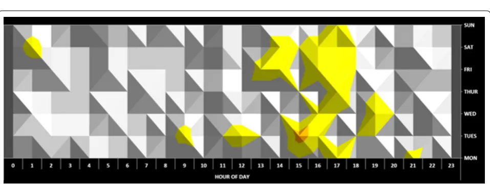
Figures 8, 9 and 10 illustrate the temporal analysis that was completed on each of the three highest robbery
Fig. 6 Robbery hot spots. Robbery hot spots and subway stations
clusters (minimum number of robberies per hot spot was 165/0.10 square mile). As you will see, there were sig-nificant temporal shifts within each of these robbery hot spots. The temporal analysis was completed using rob-bery point data that was ‘queried, clipped, and exported’ from each individual cluster and then analyzed in Micro-soft Excel (i.e. surface chart).
In the following temporal visualizations, the day of week is on the y-axis/right side of the chart (Monday at the bottom, Sunday at the top) and the time of day (mid-night on the left, to 11 pm on the right) is located on the x-axis/bottom of the chart. The color ramp varies from gray (zero/very little crime), to yellow (low crime) to dark red (very high crime). Besides the obvious temporal shifts within each cluster, it is also important to note the amount of zero/very little crime that occurs throughout each of the hot spots. This indicates the very tight tempo-ral clustering and trends that occurs within these micro-level spatial hot spots.
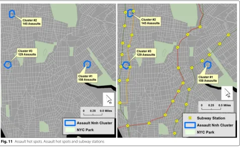
Assault hot spots
Robbery and assault are the most common forms of vio-lent crimes in the Bronx and comprise 90 % of the viovio-lent crimes in this research. Figure 5 shows the spatial dis-tribution of the three assault hot spots (each assault hot spot contains a minimum of 125 assaults per 0.10 square mile). Below is the spatial distribution of the three assault hot spots. Similar, but slightly different than robbery, it should be noted that some of the assault hot spots also intersect subway stations (Fig. 11).
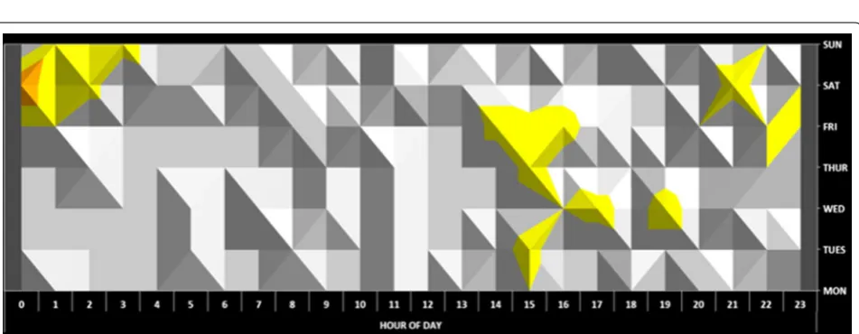
Temporal shifts within assault hot spots
Figures 12, 13 and 14 illustrate the temporal analysis that was completed on each of the assault hot spots clusters (minimum number of assaults per hot spot was 125/per 0.10 square mile). Similar to the robbery hot spots, there are also temporal shifts within each of the assault hot spots. Overall, the assault hot spots have more weekend late night/early morning temporal trends compared the robbery trends, which occur more often on weekdays and afternoons/early evenings.
Conclusion
In New York City, previous analyses conducted with NYPD (Herrmann, 2003–2012) indicate that not all vio-lent crime hot spots act the same and almost all hot spots have significant internal spatiotemporal variance. Not only do hot spots shift over time, but if crime scientists and analysts conduct temporal analysis on large scale time periods (i.e. months and years), they will notice that Table 2 Total number of crimes analyzed, minimum
num-ber of crimes per hot spot, and numnum-ber of hot spots gener-ated for the total number of crimes analyzed
Source: New York City Police Department (2011), IBM Data Warehouse/COGNOS Crime Number of crimes
(2006–2010) Minimum num-ber of crimes per cluster
Number of result-ing clusters
Robbery 22,674 165 3
Assault 20,729 125 3
crime hot spots have important temporal shifts within each hot spot. This intra-hotspot temporal variance is usually much more concentrated at more micro-levels (Ratcliffe 2004, 2006; Groff et al. 2010; Herrmann 2012).
According to the routine activities theory (Cohen and Felson 1979), crime scientists would expect to see more daytime violence patterns in geographical areas where large groups of people congregate (e.g. commercial, rec-reational, transportation areas) or where groups of people are intermingling (e.g. transportation hubs, restaurants/ bars). Nighttime violence patterns in geographical areas may be dominated by areas with higher percentages of vacant land, public transportation hubs near high popu-lation density residential areas, or commercial areas (with
late-night/24-h businesses, especially those serving alco-hol) that lack effective place managers. At more micro-levels (e.g. hot spots, hot streets, ‘risky facilities’), the Pareto Principle still remains relevant and more research should focus on micro-level variations, since these can be very beneficial when developing and implementing crime prevention and control initiatives, especially resource allocation(s) and place-management approaches.
More complex temporal analyses, such as the afore-mentioned school-day vs. non-school day robbery analy-sis, can have immediate and significant operational and administrative impacts for both crime prevention and law enforcement control programs. While we assume that there would be differences in crime patterns for these
Fig. 9 Temporal analysis of robbery cluster #2 (n = 182 robberies) shows a 5 pm–7 pm Friday and Saturday peak, as well as a weekday Wednes-day–Friday afternoon peak, between 2 pm–5 pm. Two distinct temporal patterns usually indicated two separate land-use/business establishment type robbery relationships or two separate groups of robbery offenders and/or targets. Friday are the longest crime trending days of the week, with stable trends form 1 pm–10 pm, with a prominent 5 pm–7 pm ‘rush hour’ peak
two distinct time periods (school-day afternoons vs. non-school day nights) based upon routine activity and crime pattern theory, the time–space hot spot method clearly illustrates the essential component that temporal analysis plays in our understanding of crime hot spots, especially how hot spots shift (spatially) over time and how victims,
targets, and offenders also vary according to these dis-tinct time periods.
There has been a renewed interest in this type of focus of crime at micro-level places, especially the role of place management within crime places, such as ‘risky facili-ties’. In their place management research, Madensen and
Fig. 11 Assault hot spots. Assault hot spots and subway stations
Eck (2012), suggest three new descriptions of micro-level places that take into account the ownership (i.e. ‘propri-etary’ nature of the business), the spatial clustering of places (i.e. ‘proximal’ relationships to other businesses), and the outermost boundaries or ‘pooled’ nature of the surrounding facility neighborhoods. Much of the current place management research suggests that effective place managers can have a considerable impact on the crimi-nogenic nature of risky facilities and that several preven-tion and control efforts can have a direct impact on these ‘convergent settings’ (Felson 2003) that bring people together in both time and space. By utilizing time–space hot spot techniques, place management researchers can have a much more comprehensive understanding of the different targets/victims that are at risk and how they intersect/converge with potential offenders in both time and space.
Some considerations for future research include examining the strength of the temporal patterns using circular statistics, which takes into consideration the ‘cir-cular nature’ of the 24-h time periods that are utilized in micro-level place-based research (Brunsdon and Corco-ran 2006; Wuschke et al. 2013). The process of examining spatiotemporal variations and stabilities of micro-level crime clusters can also assist crime scientists in under-standing how these micro-level place-based opportuni-ties are more generally linked to theory, which in turn can promote more effective crime prevention and control strategies and better implementation configurations.
Many of the limitations of shifting hot spots research are similar to the more generalized limitations of hot spots research; namely, the geoprocessing of crime data, the various methods of constructing crime hot spots, and the generalizability of the ‘findings’ from within the
Fig. 13 Temporal analysis of assault cluster #2 (n = 145 assaults). This cluster indicates a significant weekend and nighttime temporal pattern that is similar to assault cluster #1. There are several weekday afternoon and early evening trends (between 3 pm–8 pm) trends that occur
hot spots. Geoprocessing of crime data typically includes selecting the type(s) of crime to include in the analy-ses, selecting the appropriate time period(s) to query and analyze the crime data, and defining the appropri-ate level(s) of geographic aggregation for geocoding the crime data. While the nearest neighbor hierarchical clus-tering method provides distinct geographical boundaries, this method can also exclude relevant crime data that falls marginally outside of the crime hot spot boundary, but is still considerably related to the phenomenon being studied. Lastly, a hot spot is not a hot spot is not a hot spot… not all crime hot spots behave the same way and generalizing the spatiotemporal shifts in hot spots should be crime specific, as well as location and time specific to each respective hot spot location.
Shifting hot spots research is an important issue that merits further research in crime science and crime analy-sis. Intra-hot spot variance is good news and bad news to crime scientists and crime analysts. The good news is that many hot spots have very specific temporal ‘trends’ or definitive patterns within them, usually based on rou-tine activities, land-uses, facility types (especially ‘risky facilities’), and victim/offender schedules that are active within each hot spot. When temporal analysis is con-ducted within each hot spot, a temporal trend can nor-mally be identified and then an appropriate opportunity prevention framework, place management strategy, and/ or police response can be developed and applied. How-ever, the bad news is that if temporal analysis is not con-ducted on each hot spot, prevention resources and patrol efforts may be ineffective at best and ‘wasted’ at worst.
Competing interests
The author decalres that he has no competing interests.
Received: 26 January 2015 Accepted: 7 October 2015
References
Barnard, G. A. (1963). Discussion of Professor Bartlett’s paper. Journal of Royal Statistical Society Series B,25, 294.
Bernasco, W., & Block, R. (2011). Robberies in Chicago: a block-level analysis of the influence of crime generators, crime attractors, and offender anchor points. Journal of Research in Crime and Delinquency,48(1), 33–57. Block, C. R., & Block, R. L. (1995). Space, place and crime: Hot spot areas and
hot places of liquor-related crime. In Crime places in crime theory. Newark: Rutgers Crime Prevention Studies Series, Criminal Justice Press. Boba, R. (2001). Introductory guide to crime analysis and mapping: Report to the
office of community oriented policing services. Washington, DC: U.S. Dept. of Justice, CommunityOriented Policing Services.
Brantingham, P., & Brantingham, P. (1999). Theoretical model of crime hot spot generation. Studies on Crime and Crime Prevention,8, 7–26.
Brantingham, PL, Brantingham, PJ, Vajihollahi, M, Wuschke, K. (2009). Crime analysis at multiple scales of aggregation: A topological approach. In D. Weisburd, W. Bernasco, G. J. Bruinsma (Eds.), Putting crime in its place (pp. 87–107). New York: Springer.
Brunsdon, C. & Corcoran, J. (2006). Using Circular Statistics to Analyze Time Patterns in Crime Incidence. Computer Environmental and Urban Systems, 30, 300–319.
Bursik, R., & Grasmick, H. (1993). Neighborhoods and crime: the dimensions of effective community control. San Francisco: Lexington Books. Chainey, S., & Ratcliffe, J. H. (2005). GIS and Crime Mapping. Wiley.
Clarke, R., & Goldstein, H. (2003). Thefts from Cars in center city parking facilities: a case study. Washington, D.C.: U.S. Department of Justice, Office of Com-munity Oriented Policing Services.
Cohen, L., & Felson, M. (1979). Social change and crime rate trends: a routine activity approach. American Sociological Review,44(4), 588–608.
Dwass, M. (1957). Modified randomization tests for nonparametric hypotheses. Annals of Mathematical Statistics,28, 181–187.
Eck, J. E., & Weisburd, D. (1995). Crime Places in Crime Theory. In J. E. Eck & D. Weisburd (Eds.), Crime and Place (Vol. 4, pp. 1–33). Monsey: Criminal Justice Press.
Eck, J., Chainey, S., Cameron, J., Leitner, M., & Wilson, R. (2005). Mapping Crime: Understanding Hotspots. Washington, DC: U.S. Department of Justice, National Institute of Justice.
Eck, J., Clarke, R., Guerette, R. (2007). Risky Facilities: Crime Concentration in Homogeneous Sets of Facilities. In Crime Prevention Studies, vol. 21. Mon-sey: Criminal Justice Press.
Fagan, J., & Davies, G. (2000). Street stops and broken windows: Terry, race and disorder in New York City. Fordham Urban Law Journal. 28, 457–504. Felson, M. (2003). The Process of Co-Offending. In M. Smith, D. Cornish (Eds.),
Theory for Practice in Situational Crime Prevention, (Volume 16 of Crime Prevention Studies). Monsey: Criminal Justice Press.
Felson, M. & Boba, R.L. (2009). Crime and Everyday Life. SagePublications Inc. Glover, R. (2002). Community and Problem Oriented Policing in School Settings:
Design and Process Issues. New York: Columbia University School of Social Work.
Gorman, D., Speer, P., Gruenewald, P., & Labouvie, E. (2001). Spatial dynamics of alcohol availability, neighborhood structure and violent crime. Journal of Studies on Alcohol,2001(62), 628–636.
Groff, E. R. (2007). Simulation for Theory Testing and Experimentation: an Example Using Routine Activity Theory and Street Robbery. Journal of Quantitative Criminology,23, 75–103.
Groff, E., & McCord, E. S. (2012). The role of neighborhood parks as crime gen-erators. Security Journal,25, 1–24.
Groff, E., Weisburd, D., & Morris, N. A. (2010). Where the action is at places: Examining spatio-temporal patterns of juvenile crime at places using tra-jectory analysis and GIS. In D. Weisburd, W. Bernasco, & G. J. N. Bruinsma (Eds.), 121 Putting crime in its place: units of analysis in geographic criminol-ogy (pp. 61–86). New York: Springer.
Groff, E. R., Weisburd, D., & Yang, S.-M. (2010). Is it important to examine crime trends at a local “Micro” level? A longitudinal analysis of block to block variability in crime trajectories. Journal of Quantitative Criminology,26, 7–32.
Harries, K. (1999). Mapping Crime: Principle and Practice. Washington DC: National Institute of Justice.
Herrmann, C.R. (2012). Exploring Street-Level Spatiotemporal Dimensions of Violent Crime in Bronx, NY (2006–2010). In M Leitner (Ed.) Crime Modelling and Mapping Using Geospatial Technologies Series. Springer.
Johnson, S. D., Bernasco, W., Bowers, K., Elffers, H., Ratcliffe, J., Rengert, G., & Townsley, M. (2007). Space-time patterns of risk: a cross national assessment of residential burglary victimization. Journal of Quantitative Criminology,23, 201–219.
Kennedy, L. W., & Baron, S. W. (1993). Routine activities and a subculture of violence: a study of violence on the street. Journal of Research in Crime & Delinquency,30(1), 88–112.
Kulldorff, M. (2001). Prospective time periodic geographical disease surveil-lance using a scan statistic. Journal of the Royal Statistical Society: Series A (Statistics in Society),164(1), 61–72.
Lagrange, T. C. (1999). The impact of neighborhoods, schools, and malls on the spatia distribution of property damage. Journal of Research in Crime and Delinquency,36(4), 393–422.
Lersch, K., & Hart, T. (2011). Space, Time, and Crime (3rd ed.). Durham: Carolina Academic Press.
Levine, N. (2010). CrimeStat:A Spatial Statistics Program for the Analysis of Crime Incident Locations (v 3.3). Ned Levine & Associates, Houston, TX, and the National Institute of Justice, Washington, DC.
Madensen, T., & Eck, J. (2012). Crime Places and Place Management. In F. Cul-len & P. Wilcox (Eds.), The Oxford handbook of criminological theory (pp. 554–578). New York: Oxford University Press.
Mitchell, A. (2005). The ERSI Guide to GIS analysis, vol. 2: Spatial Measurements and Statistics. Redlands: ERSI Press.
Morenoff, J., & Robert J. S. (1997). Violent Crime and the Spatial Dynamics of Neighborhood Transition: Chicago, 1970–1990. Social Forces,76, 31–64. Newsweek. (2009). Retrieved at: http://www.thedailybeast.com/newsweek/
galleries/2009/01/17/photos-bronx-residents-on-obama.html. Newton, A., & Hirschfield, A. (2009). Violence and the night-time economy:
a multi-professional perspective. An introduction to the Special Issue. Crime Prevention and Community Safety: An International Journal, 11 (3), 147–152.
New York City Department of City Planning. (2010). Information retrieved from:
http://www.nyc.gov/html/doitt/html/consumer/gis.shtml. New York City Department of Finance. (2010). Information retrieved from:
http://gis.nyc.gov/taxmap/map.htm.
New York City Department of Buildings. (2010). Information retrieved from: https://data.cityofnewyork.us/Housing-Development/ Building-Footprints/tb92-6tj8.
New York City Police Department. (2010). New York Police Department (NYPD) Compstat Database, [Computer file, 2011].
New York City Police Department. (2011). New York Police Department (NYPD) IBM Crime Data Warehouse, [Computer file, 2011].
Ratcliffe, J. H. (2004). The hotspot matrix: a framework for the spatio-temporal targeting of crime reduction. Police Practice and Research,5(1), 5–23. Ratcliffe, J. H. (2006). A temporal constraint theory to explain
opportunity-based spatial offending patterns. Journal of Research in Crime and Delin-quency,43(3), 261–291.
Ratcliffe, J. H. (2012). The spatial extent of criminogenic places on the sur-rounding environment: a change point regression of violence around bars. Geographical Analysis,44(4), 302–320.
Rengert, G. (1997). Auto theft in Philadelphia. In R. Homel (Ed.), Policing for prevention: reducing crime, public intoxication and injury. Monsey: Criminal Justice Press.
Sampson, R., Raudenbush, S., & Earls, F. (1997). Neighborhood and violent crime: a multilevel study of collective efficacy. Science,277, 918–924. SaTScan software package (2015). http://www.satscan.org.
Shaw, C.R., & McKay, H.D. (1969). Juvenile Delinquency and Urban Areas. Rev, ed. Chicago: University of Chicago Press.
Sherman, L.W., & Weisburd, D. (1995). General deterrent effects of police patrol in crime "hot spots": A randomized, controlled trial. Justice Quarterly,12(4), 625–648.
Sherman, L. W., Gartin, P. R., & Buerger, M. E. (1989). Hot spots of predatory crime: routine activities and the criminology of place. Criminology,27(1), 27–55.
Taylor, R. B. (1997). Social order and disorder of street blocks and neighbor-hoods: ecology, microecology, and the systemic model of social disor-ganization. Journal of Research in Crime and Delinquency,34(1), 113–155. Townsley, M., Johnson, S., Pease, K. (2003). Problem Orientation, Problem
Solving and Organizational Change. In J. Knutsson (Ed.), Problem-Oriented Policing: From Innovation to Mainstream (pp. 183–212).
US Census Bureau. (2000). Retrieved from http://www.census.gov. US Census Bureau. (2010). Retrieved from http://www.census.gov. Weisburd, D., Groff, E. R., & Yang, S. (2012). The criminology of place: street
segments and our understanding of the crime problem. New York: Oxford University Press.
Weisburd, D., Morris, N., & Groff, E. (2009). Hot spots of juvenile crime: a longitu-dinal study of arrest incidents at street segments in seattle, Washington. Journal of Quantitative Criminology,25, 443–467.
Wikstrom, P.-O. H., Oberwittler, D., Treiber, K., & Hardie, B. (2012). Breaking rules: the social and situational dynamics of young people’s urban crime. Oxford: Oxford University Press.
Wilcox, P., Quisenberry, N., Cabrera, D., & Jones, S. (2004). Busy places and bro-ken windows? Toward refining the role of physical structure and process in community crime models. The Sociological Quarterly,45, 185–207. Wuschke, K., Clare, J., & Garis, L. (2013). Temporal and geographic clustering or
residential structure fires: a theoretical platform for targeted fire preven-tion. Fire Safety Journal,62, 3–12.