RESEARCH
Coordinate systems for supergenomes
Fabian Gärtner
1,2*, Christian Höner zu Siederdissen
2,3, Lydia Müller
1,3,4and Peter F. Stadler
1,2,3,5,6,7,8Abstract
Background: Genome sequences and genome annotation data have become available at ever increasing rates in response to the rapid progress in sequencing technologies. As a consequence the demand for methods supporting comparative, evolutionary analysis is also growing. In particular, efficient tools to visualize-omics data simultaneously for multiple species are sorely lacking. A first and crucial step in this direction is the construction of a common coor-dinate system. Since genomes not only differ by rearrangements but also by large insertions, deletions, and duplica-tions, the use of a single reference genome is insufficient, in particular when the number of species becomes large. Results: The computational problem then becomes to determine an order and orientations of optimal local alignments that are as co-linear as possible with all the genome sequences. We first review the most prominent approaches to model the problem formally and then proceed to showing that it can be phrased as a particular variant of the Betweenness ProBlem. It is NP hard in general. As exact solutions are beyond reach for the problem sizes of practi-cal interest, we introduce a collection of heuristic simplifiers to resolve ordering conflicts.
Conclusion: Benchmarks on real-life data ranging from bacterial to fly genomes demonstrate the feasibility of com-puting good common coordinate systems.
Keywords: Comparative genomics, Comparative transcriptomics, Big data, Graph theory, Betweenness ordering, Colored multigraph, Combinatorial optimization
© The Author(s) 2018. This article is distributed under the terms of the Creative Commons Attribution 4.0 International License (http://creat iveco mmons .org/licen ses/by/4.0/), which permits unrestricted use, distribution, and reproduction in any medium, provided you give appropriate credit to the original author(s) and the source, provide a link to the Creative Commons license, and indicate if changes were made. The Creative Commons Public Domain Dedication waiver (http://creat iveco mmons .org/ publi cdoma in/zero/1.0/) applies to the data made available in this article, unless otherwise stated.
Background
The past decade has seen rapid progress of sequencing technologies [1]. The dramatic decrease of sequencing costs has enabled an ever-accelerating flood of genomic and transcriptomic data [2] that in turn have lead to the development of a wide array of methods for data analysis. Despite recent efforts to study transcriptome evolution at large scales [3–7] the capability to analyze and integrate -omics data in large-scale phylogenetic comparisons lags far behind data generation. One key aspect of this short-coming is the current lack of powerful tools for visualiz-ing comparative -omics data. Available tools such as [8, 9] have been designed with closely related species or strains in mind. The visualizations become difficult to read for multiple species and larger evolutionary distances, where homologous genomic regions may differ substantially in their lengths, an issue that becomes more pressing the
larger regions of interest become. A common coordinate system for multiple genomes is not only a convenience for graphical representations of -omics data, however. It would also greatly facilitate the systematic analysis of all those genomic features that are not sufficiently local to be completely contained within individual blocks of a genome-wide multiple sequence alignment (gMSA).
Still, gMSAs are the natural starting point. Sev-eral pipelines to construct such alignments have been deployed over the past two decades, most prominently the tba/multiz pipeline [10, 11] employed by the UCSC
genome browser and the Enredo/Pecan/Ortheus
(EPO) pipeline [12] featured in the ensembl system. For the ENCODE project data, in addition alignments gener-ated with MAVID [13] and M-LAGAN [13] have become available, see [14] for a comparative assessment. A com-mon feature of gMSAs is that they are composed of a large number of alignment blocks. At least in the case of MSAs of higher animals and plants the individual blocks are typically (much) smaller than individual genes. As a consequence, they are not ready-to-use for detailed com-parative studies e.g. of transcriptome or epigenome [15]
Open Access
*Correspondence: [email protected]
2 Bioinformatics Group, Department of Computer Science, Universität Leipzig, Härtelstraße 16–18, 04107 Leipzig, Germany
structure. In the gMSA-based splice site maps of [16], for example, it is easy to follow the evolution of individual splice junctions as they are localized within a block. At the same time it is difficult to collate the global differ-ences of extended transcripts, which may span hundreds of blocks and to relate changes in transcript structure with genomic rearrangements, insertions of repetitive elements or deletion of chunks of sequence.
To a certain extent this problem is alleviated by con-sidering the blocks arranged w.r.t. a reference genome. For many applications, however, this does not appear to be sufficient. For sufficiently similar genomes with only few rearrangements gMSA blocks are large or can at least be arranged so that large syntenic regions can be repre-sented as a single aligned block. Any ordering of these large syntenic blocks, termed a supergenome in [17], then yields an informative common coordinate system. So far, this approach has been applied only to closely related procaryotic genomes. Prime examples are a detailed comparative analysis of the transcriptome of multiple isolates of Campylobacter jejuni [18] or the reconstruc-tion of the phylogeny of mosses from the “nucleotide pangenome” of mitogenomic sequences [19]. We remark that some approaches to “pangenomes” are concerned with gMSAs of (usually large numbers of) closely related isolates; most of this literature, however, treats pange-nomes as sets of orthologous genes [20].
Here we are concerned with the coordinatization of supergenomes, i.e., the question how gMSA blocks can be ordered in a way that facilitates comparative studies of genome annotation data. In contrast to previous work on supergenomes we are in particular interested in large ani-mal and plant genomes and in large phylogenetic ranges. We therefore assume that we have short alignment blocks and abundant genome rearrangement, leaving only short sequences of alignment blocks that are perfectly syntenic between all genomes involved. The problem of optimally sorting the MSA blocks can, as we shall see, be regarded as a quite particular variant of a vertex ordering prob-lem, a class of combinatorial problems that recently has received increasing attention in computer science [21– 24]. In the computational biology literature, furthermore, several graph-based methods have been proposed to solve the problem of sorting sequence blocks for superge-nomes, see e.g. [12, 25–29].
This contribution is organized as follows: In the follow-ing section we first analyze the concept of the superge-nome and its relationship to gMSAs in detail. We then review combinatorial optimization problems that are closely related to the “supergenome sorting problem”, and argue that the most appropriate modeling leads to a special type of betweenness ordering problem. Next, we introduce a heuristic solution that is geared towards very
large input alignments and proceeds by step-wise simpli-fication of the supergenome multigraph. Finally, we out-line a few computational results.
Theory
Genome‑wide multiple sequence alignments
Our starting point is a set of genome assemblies. For our purposes an assembly is simply a set of sequences rep-resenting chromosomes, scaffolds, reftigs, contigs, etc. In the following, we will use contig to refer to any such sequence. On each of these constituent sequences we assume the usual coordinate system defining sequence positions. Since DNA is double stranded, a piece of genomic sequence is either contained directly ( σ = +1 ) in the assembly or it is represented by its reverse com-plement ( σ = −1 ). We write (G,c,i,j,σ ) to identify the
sequence interval from positions i to j on contig c of
genome assembly G with reading direction σ . We assume,
w.l.o.g., i≤j.
Most comparative methods require multiple sequence alignments (MSAs) as input. An MSA A is
com-posed of alignment blocks, each of which consists of an alignment of sequence intervals. For the pur-poses of this paper it its sufficient to characterize an alignment block by the coordinates of its constituent sequence intervals. That is, a block B∈A has the form
B= {(Gu,cu,iu,ju,σu)|u∈rows ofB} where the index
u runs over the rows of the alignment block. It will be convenient to allow alignment blocks also to consist of a single interval only, thus referring to a piece of sequence that has not been aligned. Note that at this stage we do not assume that an alignment block contains only one interval from each assembly.
The projection πG(B) extracts from an alignment block the union of its constituent sequence intervals belonging to assembly G . If the assembly G is not represented in the alignment block B we set πG(B)= ∅.
The projection operation collapses pairs of overlapping sequence intervals ( i≤i′≤j≤j′ ) in to a single
inter-val: (G,c,i,j,σ )∪(G,c,i′,j′,σ′)=(G,c,i,j′,+1) without regard for the orientation, which is set to +1 and will have
no bearing on the algorithm we develop further down.
The projection πG of A onto one of its constitu-ent assemblies G is the union of the sequence intervals from G that are contained in its alignment blocks, i.e., πG(A)=B∈AπG(B).
Definition 1 Let A be an MSA.
• A is complete if πG(A)=G , i.e., if each position in
• A is irredundant πG(B′)∩πG(B′′)= ∅ for any two
distinct blocks B′ and B′′ , i.e., if every sequence
inter-val from assembly G is contained in at most one
alignment block.
• A is injective if no alignment block comprises more
than one interval from each of its constituent assem-blies.
Clearly, every given MSA can easily be completed by simply adding all unaligned sequence intervals as addi-tional blocks.
Just like a contig c in a (genome) assembly G , each block B∈A has an internal coordinate system defined
by its columns. We write (B, k) for column k in block B. We write ℓ(B) for the number of columns in block B. If
A is irredundant, then there are functions fG,c that map
position i within (G,c) to a corresponding MSA
coor-dinate (B, k). If A is complete, the individual fG,c can
be combined to a single function f :(G,c,i)�→(B,k) .
Completeness implies that every position (G,c,i) is
rep-resented in the MSA, and irredundancy guarantees that the relation between assembly and alignment coordinates is a function by ensuring that (G,c,i) corresponds to at
most one alignment column. The following definition is therefore equivalent to the notion of a supergenome introduced in [17].
Definition 2 An MSA A is a supergenome if it is
com-plete, irredundant, and injective.
The most commonly used genome-wide MSAs cannot be completed to supergenomes. The MSAs produced by the multiz pipeline are usually not irredundant: differ-ent intervals of the “reference sequence” may be aligned to the same interval of another assembly. While multiz
[11] alignments are injective this is in general not the case with the EPO [12] alignments. In these, multiple par-alogous sequences from the same genome may appear in one alignment block.
Now consider an MSA A and an arbitrary order < of
the alignment blocks of A . Then there is a (unique)
func-tion φ that maps the pairs (B, k) injectively to the interval [1, n], where n=
B∈Aℓ(B) is the total number of col-umns in A such that φ (B,i) < φ (B′,i′) whenever B<B′ or B=B′ and i<i′ . If A is a supergenome, then φ (f) is clearly an injective function from a genome assembly G to [1, n]. We call φ (f(G,c,i)) the coordinate of position
i of contig c of assembly G in the ordered supergenome
(A,<).
As pointed out in [17], the existence of a coordinate system for the supergenome A is independent of the
block order <. However, the order < is crucial for the practical use of the coordinate system.
Adjacency and betweenness of MSA blocks
The natural starting point for considering adjacency and betweenness of alignment blocks are their constitu-ent intervals (G,c,i,j,σ ) on a fixed assembly G and con-tig c. Intervals have a natural partial order defined by (G,c,i,j,σ )≺(G,c,k,l,σ ) whenever i<k and j<l . Two intervals are incomparable in this interval order if and only if one is contained in the other. Note that the inter-val order allows comparable interinter-vals to overlap. We also consider intervals incomparable that belong to different contigs and/or assemblies.
Given three intervals α=(G,c,i′,j′,σ′) , β=(G,c,i′′,j′′,σ′′) , and γ =(G,c,i,j,σ ) (on the same genome assembly and contig), we say that γ is between the
two distinct intervals α and β if α≺γ ≺β or β≺γ ≺α. Given a collection Q of intervals on the same assem-bly G and contig c, we say that α=(G,c,i′,j′,σ′) and β=(G,c,i′′,j′′,σ′′) are adjacent if there is no interval γ
between α and β . We say that α is a predecessor of β if α
and β are adjacent and α ≺β . Analogously, α is a a
suc-cessor of β if α and β are adjacent and β≺α.
Lemma 1 LetA be a supergenome and consider the the
collection{πG(B)|B∈A} of intervals on a givenG. Then (i)
no two intervals overlap, (ii) the interval order≺is a total
order on every contig c, (iii) every interval has at most one predecessor and one successor, and hence is adjacent to at
most two intervals, and (iv) ifγ is adjacent to bothα and
β , thenγ is betweenα andβ.
Proof Property (i) follows directly from the
condi-tion. (ii) As a consequence, any two intervals on a fixed contig c are comparable, i.e., the restriction of ≺ to c is a
total order. Since only intervals on the same contig can be adjacent, (iii) is an immediate consequence of (ii) and the fact that the number intervals is finite. Property (iv) is now a trivial consequence of the fact that by (iii) α and β must be the predecessor and successor of γ.
A key construction in this contribution is the notion of betweenness relations for alignment blocks.
Definition 3 Given three blocks A,B,C∈A , we say
that Cis between AandB with respect toG if πG(C) is between πG(A) and πG(B) . The ternary relation C (A) is the defined by (A,C,B)∈C (A) whenever C is between A and B for some assembly G.
We note that contradicting betweenness relations resulting from different genome assemblies G are to be expected, i.e., the relation C(A) will in general not satisfy
Definition 4 Two blocks A,B∈A are adjacent if there
is an assembly G such that πG(A) and πG(B) are adjacent w.r.t. {πG(C)|C∈A}.
It is useful to regard A with its adjacency relation as a
graph. In order to keep track of the individual contigs, we use an edge-colored multigraph, with G serving as edge color.
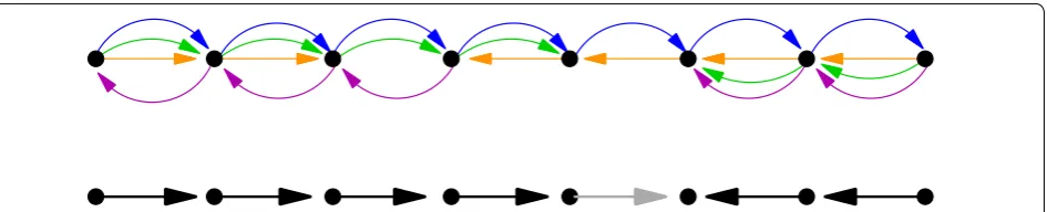
Definition 5 The supergenome graphŴ(A) of an MSA
A is the directed, edge-colored multigraph whose vertices
are the alignment blocks of A and whose directed edges
(A, B) connect an alignment block A to an alignment block B with color G whenever there are sequence inter-vals α∈A is a predecessor of β∈B in assembly G.
An example how the prejection Ŵ(A) is done is shown
in Fig. 1. The projection of Ŵ(A) to a constituent assembly
G is a (not necessarily induced) subgraph. As an imme-diate consequence of Lemma 1, each projection is a dis-joint union of directed paths, each of which represents a contig. Conversely, every colored directed multigraph
whose restriction to a single color is a set of vertex-dis-joint directed paths is a supergenome graph. It therefore makes sense to talk about a supergenome graph Ŵ
with-out explicit reference to an underlying alignment A.
The structure of the supergenome graph strongly depends on the evolutionary history of the genomes that it represents. In the absence of genome rearrangements (i.e., when the only genetic changes are substitutions, insertions (including duplications), and deletions) then all genomes remain colinear with their common ancestor. In other words, a single, canonical [30] global alignment describes a common coordinate system that is unique up to the (arbitrary) order of contigs and each trace [31] of insertions and deletions. In terms of the block adjacency relation, each block has at most two adjacent neighbors in this scenario.
Genome rearrangements are by no means infrequent events [32–35], and thus cannot be neglected. Every breakpoint introduced by a genome rearrangement oper-ation, be it a local reversal or a cut-and-join type disloca-tion, introduces an ambiguous adjacency, i.e., a block that has two or more predecessors or successors. The task of
identifying an appropriate ordering of the MSA blocks therefore is a non-trivial one for realistic data, even in the absence of alignment errors.
Modeling the “Supergenome Sorting Problem”
Informally, we may consider the “supergenome
sort-ing problem” (SSP) as the task of finding an order < (or,
equivalently, a permutation ρ ) of the alignment blocks of
Asuch that the orders of the constituent assemblies are
preserved as much as possible. Somewhat more precisely,
we are to find an order < on the vertex set of the super-genome graph Ŵ(A) that as many of its directed edges as
possible are “consistent” with the order <. It is not clear from the outset, however, how “consistency” should be defined for our application. A large number of related models have been proposed and analyzed in the literature that make this condition precise in different ways, lead-ing to different combinatorial optimization problems. We therefore proceed with a brief review of some paradig-matic approaches. A reader primarily interested in our proposed approach to the problem might want to skip this section.
Hamiltonian paths
A plausible attempt is to view the SSP as a variant of the Hamiltonian path problem on the supergenome graphŴ .
A Hamiltonian path defines a total order of the vertices and therefore a solution to the SSP. This is idea is simi-lar to the use of Hamiltonian graphs for genome assem-bly from read overlap graphs [36]. There are several quite obvious difficulties, however. First, it is not sufficient to consider only paths that are entirely confined to pass through the adjacencies. The simplest counterexample consists of only 4 MSA blocks B1 , B2 , B3 , B4 and three
assemblies G1 , G2 , G3 . Given eight sequence intervals βk,l =(Gl,ck,l,ik,l,jk,l,+1)∈Bk we construct the follow-ing alignment:
This situation arises in practice e.g. when B2 and B3 are
two independent, unrelated inserts between B1 and B4 . The block adjacency graph is the graph
which violates the desired betweenness relation
(β1,3,β3,3,β4,3).
In this case there are only two biologically correct solutions: B1<B2<B3<B4 (or the inverse order) and B1<B3<B2<B4 (or its inverse). In either case, the solution contains two consecutive blocks ( B2 and B3 ) that
B1 B2 B3 B4
g1= β1,1 β4,1
g2= β1,2 β2,2 β4,2
g3= β1,3 β3,3 β4,3
B2−B1−B4−B3,
are not adjacent in the block graph. This example also serves to demonstrate that the block graph alone does not contain the complete information on the superge-nome. It appears that in addition we will need to know
the betweenness relation among the blocks i.e., that both
B2 and B3 are between B1 and B4.
Feedback arc sets and topological sorting
An other possibility to determine a well-defined order of the vertices of the supergenome graph Ŵ is to first extract
a maximum acyclic subgraph and then to compute a topological sorting of this subgraph. An equivalent for-mulation asks for the removal of a minimum set of edges that close cycles. This Maximum Acyclic Subgraph or Minimum Feedback Arc Set problem (MFAS) is well-known to be NP-hard [37]. Nevertheless fast, practica-ble heuristics have been devised, see e.g. [38, 39]. From the resulting directed acyclic graph (DAG) an admissible ordering of blocks can be obtained efficiently by topolog-ical sorting [40]. A closely related approach is the Linear Ordering Problem (LOP): given a complete weighted directed graph, find a tournament with maximum total edge weights [41]. It yields essentially the same model since LOP and MFAS can be transformed into each other quite easily [42]. Cost functions designed to define con-sensus orderings for sets of total and partial orders have been considered in different fields starting with the work of Spearman [43] and Kendall [44], see also e.g. [45–47]. The reconciliation of partial orders in investigated in detail e.g. in [48].
The key problem of modeling the SSP in terms of MFAS is highlighted in Fig. 2. It shows that even when undirected adjacencies would allow for a perfect solution, it may not be uncovered directly by the MFAS approach.
Simultaneous consecutive ones and matrix banding
Instead of adjacencies we may consider the incidence matrix A of the supergenome graph Ŵ and try to sort both the alignment blocks and their adjacencies in such a way that, to the extent that this is possible, (i) adjacent blocks are consecutive and (ii) adjacencies that have a block in common are consecutive. In more formal terms, we wish to sort both the rows (alignment blocks) and columns (adjacencies) of the incidence matrix in such a way that rows and columns show all non-zero entries consecutively. A rectangular matrix A that admits such a pair of row and column permutations is said to have the
simultaneous consecutive ones property (C1S) [49]. This is
possible if Ŵ is a union of paths. Note that instead of
adja-cencies we could also cover the graph with short paths ℘k . In this case column k identifies the vertices incident
with path k. Again, if Ŵ is a union of paths, the
that A satisfies (C1S) if and only if A has the well-studied consecutive ones property [50, 51] for both its rows and columns. Thus (C1S) can be checked in linear time [50]. Furthermore, Tucker’s characterization of (C1S) in terms of forbidden sub-matrices [52] also carries over. Some direct connection between the consecutive ones property and the Betweenness Problem, which we will consider below, are discussed in [53].
In general, A will now have the consecutive ones prop-erty. The problem of identifying a minimal number of columns (adjacencies) whose removal leaves a (C1S) matrix is NP-complete [49]. In practise it may be desir-able to quantify the extent of the violation of (C1S) in terms of intervals of consecutive zeros enclosed by the two 1s. For instance, one may want to use ω=
ih(ℓi) ,
where the sum runs over all intervals i of consecutive zeros enclosed by the two 1s, and h(ℓi)≥0 is some con-tribution that monotonically grows with the length ℓi of
the 0-interval. For a given ordering of the rows and col-umns, the total violation is quantified as the sum of the ω values. It should be noted, however, that (C1S) does not imply Ŵ is a union of disjoint paths, i.e., that Ŵ is a valid
supergenome graph.
A related set of optimization problems is concerned with reducing the bandwidth of matrices, i.e., the maxi-mal distance of non-zero entries from the diagonal (in a symmetric case) or the parameter min(l,u)+l+u (for rectangular matrices); here u=maxAij�=0(i−j) and l=maxAij�=0(j−i) [54]. In the symmetric case, several good heuristics are known, starting with the Cuthill-McKee [55] and GPS [56] algorithms even though the problem is NP-hard [57], while the general case has received much less attention [54]. Bandwidth reduction methods do not eliminate “bad” adjacencies that eventu-ally determine bandwidth. The resulting ordering of rows and columns thus may be very inaccurate locally.
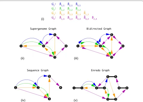
Bidirected graphs
Several specialized graph structures have been intro-duced recently to tackle the problem of ordering sequence blocks, which is a problem very similar to SSP. Among these constructions are A-Bruijn graphs, Enredo graphs, and Cactus graphs, see [58] for a review. A key insight of [58] is that these graph representations are equivalent in the sense that they can be transformed into each other. They differ, however, in additional informa-tion extracted from the input alignment that is stored as vertex and edge labels, see Fig. 3. For instance, the bidi-rected graphs of [28] have the same underlying graph as our supergenome graph. While the supergenome graph used a standard directed graph structure, bidirected graphs encode directional information independently for the endpoint of each edge, distinguishing three cases: (i) adjacent alignment blocks have the same orientation, (ii) the connected blocks switch from minus to plus orien-tation, or (iii) vice versa. The latter two cases indicate a change of orientation between two changes. In [28], this basic structure is extended by additional transitive edges given by a legal path through the graph with an exponen-tial weight function. The task is then to find a consist-ent (non-conflicting) set of edges with maximal weight. This form of the weight function takes into account that, due to genetic linkage, the more closely positioned on a genome two blocks are, the less likely it is that the edge between these blocks is broken. This gives higher weight to locally correct block positions and orientations.
syntenic order for functional reasons, such as the MHC locus used as an example in [28]. In distantly related genomes, however, synteny tends not to be well pre-served. In addition, we are interested in particular in data sets that contain genomes in preliminary draft forms, i.e., linkage information that is at least partially limited to short contigs or scaffolds. As a consequence we have less confidence in linkage and orientation information than one can expect in a typical pangenome scenario.
Sequence graphs
The sequence graphs of Haussler et al. [29] are also closely related to the supergenome graph representa-tion Ŵ(A) of a multiple alignment A . The key
differ-ence is that the the orientation of the blocks is used to
determine the direction of the edge. Two adjacent inter-vals with negative orientation thus imply an edge that is reversed compared to the supergenome graph. This situ-ation is problematic in the case where the orientsitu-ation of the intervals is switched. In [29] a preprocessing step is performed to minimize the number of such edges. The sequence graph approach was designed for the compari-son of human genomes of different individuals. In such a scenario, the resulting information loss is small and does not present a practical problem. It is likely to become an issue, however, for large phylogenetic distances with fre-quent genome rearrangements.
The natural formulation of SSP on a sequence graph is to find a vertex ordering that minimizes weighted feed-back edges and the average cut width. These optimization Fig. 3 Comparison of different graph definitions. Consider an alignment comprising of five MSA blocks ( B1 , B2 , B3 , B4 , B5 ) in four
criteria ensure that the successor relations are mostly kept intact and at the same time successors are placed close to each other in the solution. Both problems the Minimum Feedback Arc Set Problem [37] and the Average Cut-Width Minimization Problem [59–61] are known to be NP-hard. Cutwidth minimiza-tion problems ask for a linear ordering of the vertices of a graph such that the average or maximum number of edges spanning across the gap between a pair of con-secutive vertices is minimized. Conceptually, cutwidth problems are quite similar to bandwidth problems [62]. In [29] a heuristic is presented that first extracts a totally ordered “backbone” and then inserts the remaining verti-ces into the backbone order that is kept intact in the pro-cess. While the presence of a global common backbone order is a well founded assumption for pangenomes of a single or very closely related species, it is violated sub-stantially for phylogenetically diverse data.
Betweenness problems
In this work we interpret SSP as a betweenness (order-ing) problem rather than a vertex ordering problem on a directed graph. Instead of (oriented) adjacencies, which are defined on pairs of blocks, one considers the relative order of three blocks:
Betweenness Problem [63, 64]: Given a finite setX
and a collectionCof triples fromX, is there a total order
onXsuch that∀(i,j,k)∈Ceitheri<j<k or i>j>k?
This decision problem is NP-complete [63, 64]. A triple (i,j,k)∈C is called a betweenness triple.
The Betweenness Problem can be adapted to model the SSP by means of a suitable cost function b
designed to penalize violations of the betweenness rela-tion. Consider an order ρ used to coordinatize the super-genome. We may think of ρ as a bijective function from [1,. . .,|A|] →A . In other words, we number the blocks
contained in A and work on this set of block indices.
For i<j<k we set bρ,G(i,j,k)=1 if the projections of the three alignment blocks ρ(i) , ρ(j) , and ρ(k) exist and violate the betweenness relation for a given assembly G , i.e., if πG(ρ(i)) , πG(ρ(j)) and πG(ρ(k)) are located on the same contig and πG(ρ(j)) is not located between πG(ρ(i)) and πG(ρ(k)) . Otherwise we set bρ,G(i,j,k)=0 . A natu-ral cost function is now the total number of betweenness violations
where G(A) is the set of genome assemblies that are
contained in A . If genome evolution were to preserve
gene order, i.e., only local duplications and deletions are allowed, the betweenness relation of the ancestral state (1) b(ρ):=
G∈G(A)
i<j<k
bρ,G(i,j,k),
would be preserved, guaranteeing a perfect solution ρ with b(ρ)=0.
Since this decision problem is NP-complete [63, 64], so is the problem of optimizing b(ρ) NP-hard. The proof is shown in Additional file 1: Section 1 The cost function
b(ρ) involves the sum over all triples of alignment blocks and thus is fairly expensive to evaluate. It is interesting in practice, therefore, to consider a modified cost func-tion that restricts the sum in Eq. (1) to local information. This idea leads us to the rather natural extension of the Betweenness Problem to colored multigraphs.
Definition 6 Given an (undirected) colored
multi-graphŴˆ =(V,E) , the triple (i, j, k) is part of the
collec-tion C (Ŵ)ˆ , iff there are edges {i,j} ∈E and {j,k} ∈E with color G.
Colored Multigraph Betweenness Decision Problem: given the colored multigraph Ŵˆ =(V,E) , is there a total order on V such that ∀(i,j,k)∈C(Ŵ)ˆ either i<j<k or i>j>k?
The reformulation as an optimization problem that maximizes the number of edges is straightforward: Colored Multigraph Betweenness Problem: Given a colored multigraph Ŵˆ =(V,E) , find a total order on V such that E∗⊆E is maximal under the condition that ∀(i,j,k)∈C (V,E∗) either i<j<k or i>j>k.
This problem can be viewed as an analog of the Mini-mum Feedback Arc Set problem [38] for betweenness data. To our knowledge is has not been studied so far.
Lemma 2 The (decision version of the)Colored
Mul-tigraph Betweenness Problem is NP-complete.
Proof Every set C(Ŵ)ˆ of triples can be obtained from
an edge-colored multigraph Ŵˆ (with vertices ing to alignment blocks and colored edges correspond-ing to adjacencies derivcorrespond-ing from a genome identified by the color). Thus, the total order on the vertices of Ŵˆ is a solution of the Colored Multigraph Betweenness Problem if and only if the answer to the NP-complete Betweenness Problem is positive. In Additional file 1: Section 1 the reduction in both directions is shown.
In the example of Fig. 2 the optimal solution of the Colored Multigraph Betweenness Problem retains all unordered adjacencies and creates a unique coordinatization (up to orientation) that leaves all align-ment blocks ordered as drawn.
Seriation
Robinson seriation problem [65] starts from a dissimilar-ity measure d:X×X→R , and seeks a linear order ρ on
X that satisfies the inequality
A dissimilarity d for which an ordering ρ exists that
sat-isfies Eq. (2) for all ρ(i) < ρ(j) < ρ(k) is called Robinso-nian. It is worth noting that Robinsonian dissimilarities are intimately related with pyramidal clustering problems [66, 67].
The seriation problem [65, 68] consists of finding a total order for which the given pairwise distances vio-lates the Robinson conditions as little as possible. To link this seriation problem with the Colored Multigraph Betweenness Problem or Betweenness Problem we consider a collections C of triples such that
Clearly, if the dissimilarity is Robinsonian, then ρ defines
a total order on X that solves the Betweenness Prob-lem for (X,C).
The relevant optimization task in our context is there-fore to minimize the number of ordered triples that vio-late Eq. (2). A variety of heuristics for this problem have been developed, see e.g. [69]. It is important to note, however, that in our setting the distance between align-ment blocks is not defined directly. In order to obtain a seriation problem that approximates the Supergenome Sorting Problem we will have to resort to a heuristic that summarizes the distances between two blocks in all genomes and reflects the betweenness relationships. For pangenome-like models, the cost function advocated in [28] is a very plausible choice.
Graph simplification
Each of the plausible models for the “Supergenome Sort-ing Problem” discussed in the previous sections leads to NP-hard computational problems. The size of typi-cal genome-wide alignments by far exceeds the range where exact solutions can be hoped for, except possibly for the smallest and most benign examples such as the ones used as examples in [17]. We therefore will have to resort to fast heuristics. In this section we focus on the conceptual ideas behind the simplification steps. More detailed implementation details are given in the " Meth-ods" section.
Nevertheless it is possible to isolate certain sub-prob-lems that can be solved exactly and independently of the remainder of the input graph. Since “linearized” portions of the vertex set can be contracted to a single vertex set, this leads to a reduction of problem size.
(2) max{d(ρ(i),ρ(j)),d(ρ(j),ρ(k))} ≤d(ρ(i),ρ(k)).
(3) (ρ(i),ρ(j),ρ(k))∈Cimplies max
{d(ρ(i),ρ(j)),d(ρ(j),ρ(k))}<d(ρ(i),ρ(k))
Lemma 3 If the supergenome graphŴ is a directed
acy-clic graph then topological sorting ofŴ solves theColored
Multigraph Betweenness Problem.
Proof In this case betweenness is established exactly
by the directed paths in the DAG. Hence any topologi-cal sorting preserves all betweenness triples of G and thus presents a perfect solution to the Colored Multi-graph Betweenness Problem as well.
This simple observation suggests to identify subgraphs with DAG structure and to replace them with a rep-resentative for each replaced DAG. These can later be replaced by the solution that is created with topological sorting. We note that this does not necessarily preserve optimality. It is conceivable that a local DAG structure has to be broken up into two disjoint subsets that are integrated in larger surrounding structures in a way that requires reversal of the edge directions in one or even both parts. Nevertheless, if the local DAG structures are sufficiently isolated they are likely to be part of the opti-mal solution as a unit. The motif that describes such a local DAG structure has been introduced as “superbub-ble” in the context of graph structures arising in sequence assembly problems [70, 71].
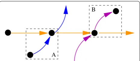
Source and sink vertices s in the supergenome graph with only a single neighbor t are conceptually a special case of superbubbles. These can be sorted together with their unique neighbor t. Ŵ is thus simplified by
contract-ing s and t, i.e., placing the source s immediately before t
and sink s immediate after t. An example of such a source and a sink can be seen in Fig. 4.
In some cases it is helpful to reverse the direction of the coordinate system of a single species. This is in par-ticular the case when a single genome is reversed com-pared to all others. The inversion of an entire path does not change the solution of the Colored Multigraph
B
A
Betweenness Problem but can make it easier to apply some of the reduction heuristics discussed above. In par-ticular, if the relative orientation of the coordinatizations could be fixed in an optimal manner, the betweenness problem reduces to a much easier topological sorting problem. Finding this optimum, however, is equivalent to the Betweenness Problem, which is a NP-hard. Hence, we again have to resort to local heuristics.
Definition 7 Let Ŵ=(V,E) be a supergenome graph. A pair of vertices v,w∈V such that there are edges (v, w) and (w, v) in E is a mini cycle.
Mini-cycles are naturally removed by removing one of the two edge directions between v and w. More precisely, the less supported direction of an edge is dropped. The estimate for support is evaluated in a region around a mini-cycle since adjacent mini-cycles may yield contra-dictory majority votes.
Definition 8 Two mini-cycles are connected with each other if they share a vertex. A mini-cycle complex C is a maximal connected set of mini-cycles.
Lemma 4 The mini-cycle complexes of a supergenome
graphŴ form a unique partition of the set of all
minicy-cles. Any two classes of this partition are vertex and edge disjoint.
Proof Consider the the graph H whose vertices are
the mini-cycles, and there are edges between any two mini-cycles that share at least one vertex. Then every mini-cycle complex C is a connected component of H. Since the connected components of a graph are uniquely defined, disjoint, and form a cover, they partition the vertex set of H. Every minicycle, furthermore, forms a connected subgraph of Ŵ by construction. Since any two
minicycles that contain a common vertex belong to the same mini-cycle complex, two mini-cycle complexes can-not have a vertex in common. This implies that they are also edge disjoint.
The mini-cycle complexes therefore can be resolved independently of each other. The target is to remove edges that create cycles in order to obtain a DAG that can then be subjected to topological sorting. However, this topological sorting is a solution of the Colored Multigraph Betweenness Problem for a subgraph. This is still a hard problem, so that we again utilize a heu-ristic approach. In this step we only attempt to remove mini-cycles. Cycles that connect mini-cycle complexes with each other or with other vertices in the graph are
therefore left untouched and have to be dealt with in a subsequent step.
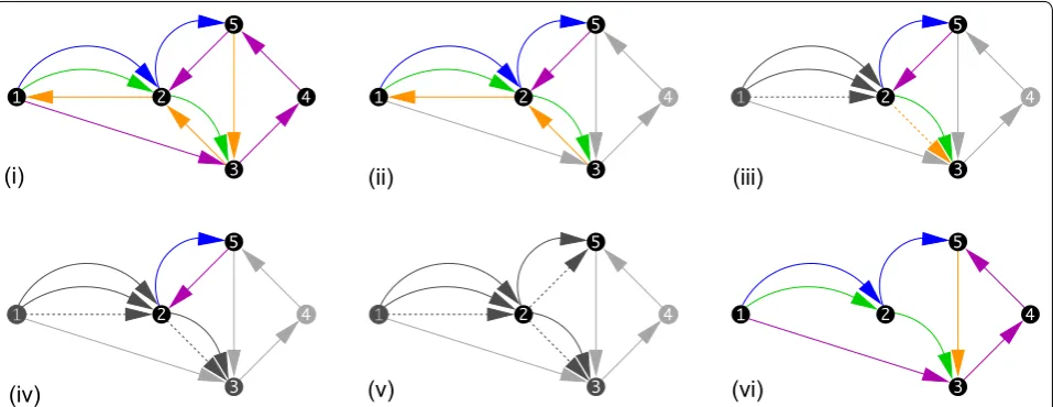
The local sorting within a complex C is achieved by con-sidering adjacencies. To this end we annotate each adja-cency with the number of edges and the ratio of the edges in the two directions. We identify the best supported edges as those with a high multiplicity and a strong bias for one direction over the other. This choice of a direction is then propagated. If a directed edge has more than one possible successor, we first propagate along the one with the largest support for the proposed direction. The issue now is when exactly to stop propagating this information. Clearly, it is forbidden to orient an edge that would close a directed cycle. Any such edge is instead seeded with the reverse directional information.
As part of this procedure it is possible that parts of a directed path from a given genome received contradic-tory orientations in different regions. If this is the case, the edge crossing the boundary between the differently oriented regions must be removed. Finally, the heuris-tic may terminate and still leave some edges unoriented. This indicates that the orientations are contradictory and need to be reversed. An example of the mini-cycle reso-lution process is shown in Fig. 5.
Methods
Curation of input data sets
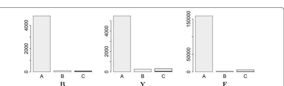
We investigate here three genome-wide data sets. The smallest set, referred to as B (bacteria) below, is an
alignment of four Salmonella enterica serovars. This alignment was produced with Cactus [27] using the
Sal-monella enterica Newport genome as reference and
com-prises 13, 416 blocks, 50, 932 sequence fragments, and 18, 047, 456 nucleotides. The medium-size set, termed Y
(yeast), is an alignment of seven yeast species that uses
the Saccharomyces cerevisiae genome as references.
It comprises 49, 795 alignment blocks composed of 275, 484 sequences fragments that contains 71, 517, 259 nucleotides. The third, much larger set F (fly) is a align-ment of 27 insect species that uses the Drosophila
mela-nogaster genome as references. It comprises 2, 112, 962
blocks composed of 36, 139, 620 sequence fragments hat contains 2, 172, 959, 429 nucleotides. For more detailed information of the data sets refer to Additional file 1: Section 2.
inserted to bridge gaps between larger blocks. Conse-quently, they convey little or no useful information for our purposes. We therefore remove all blocks with a length ≤10 nt.
Since genome-wide alignments tend to contain also very poorly aligned regions we require a minimum similarity, expressed here in the form of sum-of-pairs
blastz scores [73]. Since these scale linearly with the number of columns ℓ(B) of the alignment block B and the number
r
2
of pairwise alignments formed by the r
rows in B, we normalize with
r 2
ℓ(B) to obtain a simi-larity measure that is independent of the size of the align-ment block. Based on the parametrization of blastz, we set the threshold at a normalized score of −30 , which
corresponds to the gap extension penalty.
The coordinatization of the supergenome depends on the uniqueness of coordinate projections. There are three major reasons to observe overlaps, i.e., genomic regions that appear in more than one alignment: (i) the sequence is duplicated in some species. Then multiz
tends to align the corresponding unduplicated sequence to both duplicates. (ii) Spurious similarities in particular in poorly conserved regions may lead to alignments con-taining a sequence element twice at the expense of the second copy. (iii) Short overlaps at the end of blocks may appear due to difficulties in determining the exact ends of alignable regions. The first two causes introduce unde-sirable noise and uncertainties. Therefore, we remove all
such overlapping blocks in which sequences from the species overlap. Since there is no easy way to determine which one of two overlapping blocks is likely correct, we opt to remove both copies. The third case, in contrast, does not disturb the relative order of alignment blocks and thus can be ignored. The overlap filter is applied after low quality alignments already have been removed from the data set.
We tolerate an overlap of 20 nt at the borders of align-ment blocks. This cutoff is designed to remove ambigu-ous alignments, while avoiding the removal of alignment blocks that overlap by a few nucleotides owing to over-lapping extensions of local blastz seeds. In addition we remove sequences that completely overlap other sequences regardless of their size to further reduce the noise introduced by spurious alignments. We opt here for a stringent procedure and remove all alignment blocks that contain sequences tagged for removal. In practice, this step removes only a tiny fraction of the blocks and thus does not significantly influence the coverage of the retained data.
The initial data filtering steps removed almost 35%
( 40% , 30% ) of the blocks from data set F , ( Y , B ). The
majority were eliminated because of their minimal length. About 8.5% ( 27% , 0% ) of the blocks were removed because they contained non-unique sequences. The sequences in the blocks that are removed with all filters contain less then 15% ( 26% , 0.4% ) of the nucleotides in the alignment. Hence more than 85% ( 74% , 99% ) of the
sequence information of the alignment is intact and the quality of the data is significant better. A more detailed summary of the filtering is compiled in Additional file 1: Section 2.
Graph simplification and DAG construction
The algorithmic ideas and their justifications for the graph reduction steps have already been discussed in "Theory" section. Here we briefly address implementa-tion issues as well as particular choices of cost funcimplementa-tions and parameters that were discussed in a more general setting above.
The filtered data is used to create an initial superge-nome graph. Then we iterate the three different graph simplifiers until no further reduction steps can be applied: the mini-cycle remover, the source/sink sim-plifier, and the superbubble simplifier. The individual simplifiers are straightforward implementations of the basic ideas outlined above. The mini-cycle remover first identifies the mini-cycles, aggregates them into non-overlapping complexes, and then proceeds to remove contradictory edges in a greedy manner. The other two simplifiers first check for each vertex in the input graph whether it is a valid sink, source, or starting vertex of a superbubble. Pseudocode of the simplifiers is given in Additional file 1: Section 4.
The mini-cycle remover works more effectively on a single big complex than on many small ones separated
by narrow gaps. The other two simplifiers therefore are applied until a fixed point is reached to close some of these gaps. The entire procedure is then iterated until the minicycle remover cannot change the graph any further.
Once a fixed point is reached we attempt to remove directed cycles. This amounts to solving the Minimum Feedback Arc Set Problem, which is known to be NP-hard [37]. Given the size of our input graphs we have to resort to linear-time heuristics. We use Algorithm GR [38] because it is known to work particularly well on sparse graphs. Cycle removal typically creates new pos-sibilities to simplify the graph. For instance, a sink is created whenever the last outgoing edge of a vertex is removed. The new sink can then be simplified further. The graph simplifiers are therefore applied again after the cycle removal step.
The minicycle remover is not used in this second pass because it is not applicable to DAGs by construction. Instead, we use a generalized version of the source/sink simplifier in which a source s may have more than a sin-gle successor v, provided v is a predecessor of all other successors of s. The position of source s in the DAG is determined by v and thus s can be placed immediately before v. The corresponding arrangements for a sink and its predecessor is treated analogously.
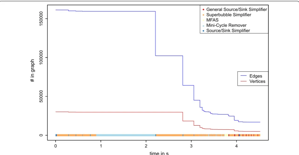
The running time and the minimization of the data set while this process is applied is shown in Figs. 6, 7 and 8.
time in s
#i
n
grap
h
0.0 0.2 0.4 0.6 0.8 1.0
0
200
04
00
06
000
8000
10000
S MFAS
Mini-Cycle Remover Edges
Vertices
Seriation
Finally, the common coordinate system is created by seri-ation of the DAG. The resulting supergenome, i.e. linear order of the vertices of the graphs corresponds to a lin-ear order of all blocks. In particular, vertices resulting from a simplifier may contain more than one block. Those blocks, however, are already sorted and thus are inserted as a single block. Seriation is naturally divided into two steps. First, topological sorting is used to calculate an ini-tial linear ordering from the DAG. Kahn’s algorithm [40] is a classical solution to the topological sorting problem. For our purposes it is desirable that, if possible, two nodes
v and w are placed consecutively whenever there is an edge (v, w) in the final DAG. To this end we modify Kahn’s algorithm by sorting the successors of a node in the order of evidence for their adjacency in the original data.
The order obtained in this manner may not be optimal w.r.t. its agreement with the order of the blocks in the genomes. It provides a good starting point, however, for the final optimization step, which we phrase as minimiz-ing the number τ of triplets (i, j, k) for which the Rob-inson condition, Eq. (2), page 12, is violated. We use the distance measure
(4) d(i,k)=
1
|(i,k)| if an edge(i,k)exists,
mini<j<k{d(i,j)+d(j,k)} if a path from i to k through j exists,
∞ if no path from i to k exists,
where |(i, k)| is the number of edges from i to k. Since d
is a good measure of co-linearity only for short distances, we limit the path length in Eq. 4 to a small number of l
edges. We set l=10 in our implementation. In addition this reduces the effort of computing the distances from O(|V|2) to O(|V|) as a consequence of the sparsity of the
input graph.
We use a gradient descent-like optimization algorithm to minimize τ . We say that two nodes are siblings if they either share a predecessor in the DAG or if they are both sources. The move set for the gradient descent consists of swaps of siblings only. In addition, we allow to move a node directly in front of its sibling. The discrete gradient is computed exhaustively by generating and evaluating each potential move. Since non-overlapping swaps do not influence each other, we greedily execute a maximal set of non-overlapping swaps in a single optimization step.
Assessment of the quality of supergenome coordinate systems
Since no ground truth is available for this problem and the construction of simulated benchmarks for genome wide multiple sequence alignments would be a research
0 1 2 3 4
0
50000
100000
150000
time in s
#i
ng
raph
Edges Vertices MFAS
Mini-Cycle Remover
project in its own right, we have to resort to measuring quantities that are informative about the final choice of the coordinate system.
A straightforward measure is the distribution of dis-tances in the output coordinate system of alignment
blocks that are contiguous in at least one input genome. Since we are not interested in the length of align-ment blocks, distance is measured here not in terms of sequence length but in terms of the number of align-ment blocks, so that adjacent blocks have distance 0. It
time in s
7900 8000 8100 8200
0
2000000
4000000
6000000
8000000
1000000
0 1200000
0
#i
n grap
h
0 2000 4000 6000 8000
time in s
0
500000
01
000000
01
500000
02
000000
02
500000
0
#i
n
grap
h
S MFAS
Mini-Cycle Remover Edges
Vertices
is important here to keep track of the reading directions: contiguity with the same reading direction corresponds to preservation of the original genomic coordinates, while a change in reading direction indicates change of the order. Thus we distinguish preserved and inverted reading direction in our quantitative analysis.
Open reading frames (ORFs) are among the best-con-served features in the genome due to the strong selection pressures acting to preserve the corresponding proteins. As an immediate consequence we expect that ORFs are almost always preserved. This should be reflected also by the supergenome coordinates, i.e., blocks belonging to the same ORF should have only a small number (smaller then 5) of other blocks between them and retain their relative order. For higher eukaryotes, we cannot expect near perfect adjacency of coding blocks, however, because larger introns are subject to local rearrangements. To quantify the prox-imity of blocks of an ORF, the distances between all adja-cent blocks are determined as described above and their absolute values are added up to yield a single characteristic value. In addition we count the number of exons that are “broken up” in the sense that consecutive pieces do not have consecutive coordinates or are placed in reverse order in the supergenome. Coding genes and exons are taken as annotated for the corresponding genomes. We note that in particular for large, intron-rich genomes such as the insect data set F this is an additional source of errors.
Results and discussion
We have devised a heuristic algorithm to extract a com-mon coordinate system for a supergenome from a genome-wide multiple sequence alignment. The proce-dure has been tested on three alignments of very differ-ent size and difficulty: an easy instance comprising four closely related bacterial species, an intermediate size problem composed of seven yeast genomes, and the align-ment of 27 insect genomes as the most difficult instance.
Performance of individual components
The heuristic algorithm outlined above is composed of several largely independent components. It is of inter-est, therefore to consider their relative impact on the final results. We find that most edges are removed by the mini-cycle remover, with a small contribution of Algo-rithm GR. On the other hand, the largest reduction of the vertex set is due to the merges identified by the closed DAG simplifier. More quantitative information is compiled in Figs. 6, 7 and 8 and in Additional file 1: Sec-tion 8. The simplifiers reduce the graph size by about an order of magnitude in both the number of vertices and edges, reducing it in size and complexity to a point where the seriation heuristic operates efficiently. The relative improvement is smallest for the bacterial data set.
Since the Colored Multigraph Betweenness Problem cannot be solved exactly in reasonable time for instances with sizes that are of interest for our applica-tion at hand, we cannot measure performance relative to the exact solution. The multigraphs obtained from real-life alignments contain a large number of conflicting edges. In the most difficult data set, F , for instance, the final order keeps more than 95% of the initial edges.
Quality of supergenome coordinate systems
The quality of the coordinate systems strongly depends on the quality of the input alignments. A detailed discus-sion of issues with the input alignments can be found in Additional file 1: Section 8. Here, we focus on an assess-ment of the coordinate systems themselves.
In order to check the overall quality of the solution we compute a betweenness graph from the superge-nome coordinate systems. This is done by starting with a graph without edges. First, all edges that are supported by the total order of the supergenome are added. This is followed by edges that contradict the total order but do not create contradicting betweenness triples. Note that this graph is not necessary optimal but a good approxi-mation that can easily be computed. The edge set of this graph is compared to the edge set of the initial graph. Good solutions are expected to retain most of the edges. For the three data sets we find that 95.3%, 97.5%, and 99.4% of the edges are retained in data sets B , Y , and F , respectively.
The distribution of block-wise distances in the super-genome of alignment blocks that are consecutive in the original genome serves as a simple measure of pre-served synteny. The results are summarized in Fig. 9 and presented in full detail in Additional file 1: Section 8. Another measure is how many of the input orders are preserved. To measure this we consider every alignment block and all successors from the different genomes. For the bacterial data set B89% of the successors preserve the
order and 80% also preserve the adjacency. For the yeast data set Y we observe that 93% of the successors
are meaningful and indeed are likely a useful starting point for large-scale multi-genome comparisons.
Restricting our attention to coding sequences yields a more stringent quality measure, as shown in Fig. 10. As bacteria have essentially no introns, we expect that nearly all blocks belonging to the same ORF retain both adja-cency and order. In the bacterial data set B96% of the
ORFs are in one stretch with no interruption and less then 1% of the ORFs are broken. Since yeasts have few and short introns [74] we expect that data set Y is also
very well-behaved in this respect. It contains 6062 ORFs annotated for Saccharomyces cerevisiae. Of these, 5474, i.e., 90% , are consistently represented in the coordinate system. An additional 272 ORFs, about 5% , have a
dis-tance of less then 100 blocks between them. Only 73, i.e.,
a bit more than 1% of the ORFs are broken. For
Drosoph-ila melanogaster are 167, 051 exons annotated, and part
of the alignment F . Due to large and abundant introns the analysis is based on individual exons rather than com-plete ORFs for set F . We observe that 95% of the ORFs/ exons are consistently represented. Only 779, about 0.5% ,
are broken. Overall, thus, the supergenome coordinates behave very well for all three data sets.
As a specific example we consider the genes of the yeast TCA cycle [75] in more detail. It is one of the best-stud-ied enzyme systems and known to be essential in S.
cer-evisiae. There, it comprises 20 genes [76–79], all of which
are contained at least partially in the initial set of align-ment blocks in the yeast data set Y . Only nine genes are
included in their entirety, however. Seven of these nine
- +
-A
+
-A
C B A A B C C B A B C C B A B C
0
5000
15000
25000
0
50000
100000
150000
0
5000000
15000000
+
B Y F
Fig. 9 Distribution of block-wise distances of consecutive alignment blocks in the original genomes. Data are shown separated for inverted (−) and preserved (+) orientation of consecutive blocks (light gray). As expected, the number of inverted blocks increases with the difficulty of the input alignment. In particular, there is a substantial number of local inversions in the insect data set F . Both the inverted (−) and preserved (+) bin are subdivided further into a bin of adjacent blocks (A), blocks with a distance of 1–5 blocks (B), and more distantly placed blocks (C), in the superge-nome
are represented colinearly in single blocks. The align-ments for KGD2 and SDH2 cover multiple MSA blocks and there is intervening genomic sequence in the input alignment, leading to non-contiguous placement in the final coordinate system. The alignment blocks referring to the remaining 11 genes are difficult to analyze and may contain misassigned sequences. This example, similar to several other loci, suggests that the quality of the input alignment rather than the complexity of the between-ness problem is the limiting factor for the construction of supergenome coordinate systems.
Conclusion
In this contribution we have shown that the problem of computing a common coordinate system for superge-nomes with the Colored Multigraph Betweenness Problem is NP-hard. It belongs to a class of relatively poorly studied betweenness problems for which few effi-cient heuristics have been developed so far. We intro-duced here several local simplification rules that can be applied iteratively to reduce the problem. It is important to note these reduction steps are only heuristics and do not guarantee optimal solutions. In conjunction with a simple serialization approach for the residual graph, they nevertheless yield practically useful results with accept-able computational efforts.
The most immediate application of the supergenome sorting problem is the direct comparison of genome annotations for multiple genomes. Hence it constitutes a prerequisite for comparative genome browsers. We have applied our approach to three real-life data sets of differ-ent sizes and difficulties. Our results indicate that prac-tically useful coordinatizations can be computed. The computational requirement of the method scales favora-bly so that in principle even the largest genome-wide multiple sequence alignments could be processed.
The present study, however, also highlights the short-comings of currently available genome-wide multiple sequence alignments [80, 81]. The issue is not only the relatively moderate coverage with alignment blocks that contain at least most of the species under consideration, but also the substantial fractions of alignment blocks that have been removed from our data set due to likely arte-factual sequences. We have therefore not attempted to analyze the UCSC 100-way vertebrate alignments, since these data are even more complex than the insect data due to the very large number of paralogs introduced by genome duplications.
Synteny, i.e., the preservation of relative genome order, is in general a good predictor for homology. This fact suggests to use the common coordinate system to iden-tify likely homologous regions that are not included in the initial alignment blocks. These could then be (re)
aligned at sequence level and included in a revised mul-tiple sequence alignment. This, in turn, could yield an improved common coordinate system. The systematic improvement of genome-wide alignments, albeit an interesting and extremely useful endeavor, is beyond the scope of this contribution.
Possible improvements of the approach taken here are conceivable in at least two directions. First, one may consider a hybrid algorithm that solves subgraphs with a dominant backbone use the method discussed in [29]. As discussed, we assume that large parts of the global graph structure are not amenable to such a solution, but it is also reasonable to assume that gene regions under strong conservation pressures can be solved fairly easily using a local backbone-based approach. A second venue of research is concerned with the determination of the final backbone order. Depending on the phylogenetic range under investigation, the ancestral gene order would provide a useful backbone based on the phylogeny of the species involved in the alignment.
Authors’ contributions
CHzS and PFS designed the study, FG and LM implemented the software and performed the computational analysis. All authors collaborated on the design of the algorithms and the overall work flow, the interpretation of results, and the writing of the manuscript. All authors read and approved the final manuscript.
Author details
1 Competence Center for Scalable Data Services and Solutions Dresden/ Leipzig, Universität Leipzig, Augustusplatz 12, 04107 Leipzig, Germany. 2 Bioinformatics Group, Department of Computer Science, Universität Leipzig, Härtelstraße 16–18, 04107 Leipzig, Germany. 3 Interdisciplinary Center for Bio-informatics, Universität Leipzig, Härtelstraße 16–18, 04107 Leipzig, Germany. 4 Automatic Language Processing Group, Department of Computer Science, Universität Leipzig, Augustusplatz 12, 04107 Leipzig, Germany. 5 Max Planck Institute for Mathematics in the Sciences, Inselstraße 22, 04103 Leipzig, Ger-many. 6 Department of Theoretical Chemistry, University of Vienna, Währinger Straße 17, 1090 Vienna, Austria. 7 Center for non-coding RNA in Technology and Health, Grønegårdsvej 3, 1870 Frederiksberg C, Denmark. 8 Santa Fe Institute, 1399 Hyde Park Rd., Santa Fe, NM 87501, USA.
Acknowledgements
This work was funded by the German Federal Ministry of Education and Research within the project Competence Center for Scalable Data Services and Solutions (ScaDS) Dresden/Leipzig (BMBF 01IS14014B). We acknowledge support for APCs from the German Research Foundation (DFG) and Universität Leipzig within the program of Open Access Publishing.
Competing interests
The authors declare that they have no competing interests.
Consent for publication
Not applicable. Additional file