Stochastic errors vs. modeling errors in distance based phylogenetic reconstructions

R E S E A R C H

Open Access

Stochastic errors vs. modeling errors in

distance based phylogenetic reconstructions

Daniel Doerr

, Ilan Gronau

, Shlomo Moran

and Irad Yavneh

Abstract

Background: Distance-based phylogenetic reconstruction methods use evolutionary distances between species in order to reconstruct the phylogenetic tree spanning them. There are many different methods for estimating distances from sequence data. These methods assume different substitution models and have different statistical properties. Since the true substitution model is typically unknown, it is important to consider the effect of model misspecification on the performance of a distance estimation method.

Results: This paper continues the line of research which attempts to adjust to each given set of input sequences a distance function which maximizes the expected topological accuracy of the reconstructed tree. We focus here on the effect of systematic error caused by assuming an inadequate model, but consider also the stochastic error caused by using short sequences. We introduce a theoretical framework for analyzing both sources of error based on the notion ofdeviation from additivity, which quantifies the contribution of model misspecification to the estimation error. We demonstrate this framework by studying the behavior of the Jukes-Cantor distance function when applied to data generated according to Kimura’s two-parameter model with a transition-transversion bias. We provide both a

theoretical derivation for this case, and a detailed simulation study on quartet trees.

Conclusions: We demonstrate both analytically and experimentally that by deliberately assuming an oversimplified evolutionary model, it is possible to increase the topological accuracy of reconstruction. Our theoretical framework provides new insights into the mechanisms that enables statistically inconsistent reconstruction methods to outperform consistent methods.

Keywords: Phylogenetic reconstructions, Substitution models, Additive substitution rate functions

Introduction

Phylogenetic reconstruction is the task of determining the topology of an evolutionary tree underlying a given set of samples (species) using sequence data extracted from them. This is typically done by assuming some simpli-fied model for DNA sequence evolution, in most cases modeling it as a homogeneous continuous-time Markov process [1-3]. Distance-based reconstruction algorithms tackle this task by first computing a set ofn₂pairwise dis-tances between theninput samples and then finding a tree which fits these distances. The distance measures used for this purpose typically reflect the rates of certain substitu-tion events along the evolusubstitu-tionary paths in quessubstitu-tion. We

*Correspondence: [email protected]

3Computer Science Department, Technion - Israel Institute of Technology, Haifa, Israel

Full list of author information is available at the end of the article

thus refer to these distance measures assubstitution rate (SR) functions. The distance-based approach is based on the fact that if the SR function used is additivefor the underlying substitution model, and the input sequences are sufficiently long, then the topology of the true tree can be efficiently recovered with high probability. How-ever, since the underlying evolutionary model is usually unknown, this assumption is rarely satisfied in practice.

Substitution models used for phylogenetic reconstruc-tion range from the simplest Jukes-Cantor (JC) model [4], through slightly more complex and flexible mod-els, such as Kimura’s two-parameter (K2P) model [5] and the Hasegawa-Kishino-Yano model (HKY) [6], to the General Time-Reversible (GTR) model [7,8]. In previous works [9,10] we observed that substitution models which are not too restrictive or too general have many inherently different additive SR functions.

We used this basic observation to demonstrate that it is possible to adjust for each given set of DNA sequences a “good” additive SR function, which leads to signif-icantly increased phylogenetic reconstruction accuracy, compared to other additive SR functions. This exploits our ability to predict thestochastic noiseassociated with each SR function. When the SR function used for dis-tance estimation is additive for the underlying substitution model, this stochastic noise is the only cause for inaccu-rate reconstruction. However, in the scenario, which is very common in practice, where the SR function in use is not additive for the model, an additional systematic bias is introduced in the distance estimates. This systematic bias in distance estimation results in a phylogenetic recon-struction method that might be statistically inconsistent in some cases. In this papera, we extend our previous line of research to this scenario, by removing the constraint of additivity. We do this by considering both the stochastic noise and systematic error.

Several previous studies have demonstrated the util-ity of phylogenetic reconstruction methods that are not generally statistically consistent. The maximum parsi-mony method has been long known to be inconsistent in some cases [11,12]. However, in other cases it was shown to be more likely to produce accurate reconstruc-tions, compared with the maximum likelihood method [13-15]. More recently, it has been demonstrated that reconstruction accuracy can be improved by deliberately assuming an oversimplified substitution model, when reconstructing a tree using maximum likelihood [16,17]. In the context of distance-based reconstruction, non-additive distance measures have been shown in several cases to lead to improved accuracy when compared with additive measures [18,19]. Overall, these studies provide convincing evidence for the need to consider incon-sistent phylogenetic reconstruction methods. However, none of them provide a rigorous framework for character-izing the cases in which inconsistent methods outperform consistent ones.

In this paper we develop a theoretical framework which provides a practical and systematic way to quantify the effect of distance-estimation-bias on the accuracy of distance-based reconstruction. This framework is based on a novel method for measuring thedeviation from addi-tivity of SR functions. Coupled with the results in [9], this method enables evaluation of both the systematic bias and stochastic noise of SR functions. Such evaluation is important, because there is often a tradeoff between these two sources of error, stemming from the fact that simpler models with fewer parameters (such as JC) have smaller stochastic noise at the expense of greater estimation bias. Our framework allows us to consider this tradeoff when deciding which SR function to use for a given data set. This allows us to characterize a wide range of cases in

which an SR function associated with an oversimplified evolutionary model results in increased reconstruction accuracy.

This finding falls in line with previous studies demon-strating the usefulness of phylogenetic reconstruction methods that are not generally consistent. Previous stud-ies have attributed the increased accuracy of inconsis-tent methods mainly to the fact that these methods have a bias toward reconstructing certain topologies, leading to increased accuracy in cases where the phy-logeny being reconstructed has the “favored topology”. We notice a similar behavior using our theoretical characterization of non-additive SR functions. However, somewhat surprisingly, we find that non-additive SR functions often have an advantage even when the phy-logeny being reconstructed has an “unfavorable topol-ogy”. This is due to the reduced stochastic noise of the non-additive SR function (compared with it addi-tive alternaaddi-tives), which compensates for its topological bias.

Our paper is organized as follows. Section “Background” outlines some of the required background and introduces several new concepts that are central in our analysis. Section “Deviation from Additivity in Homogeneous Sub-stitution Models” provides the main analytic results in the paper, and introduces deviation from additivityas a measure of distance estimation bias. In that section we prove a general upper bound for this deviation and estab-lish a connection with reconstruction accuracy. We then study deviation from additivity and stochastic error of the JC distance formula when applied to data generated under the K2P model. In Section “Performance of Non affine-additive SR Functions in Quartet Resolution” we study the effect of deviation from additivity and stochas-tic error on the accuracy of quartet reconstruction. In the case of quartets we can draw a tight connection between the different sources of error in distance estimation and inaccuracy of reconstruction. We present a useful heuris-tic, based on the so-called Fisher criterion ([20,21]), for comparing the expected accuracy of two SR functions in this context. In Section “Simulations on Hasegawa’s Tree” we extend our study to larger trees using experiments on simulated data based on the tree obtained by Hasegawa in [6]. Finally, In Section “Inferring Trees from Genomic Sequences” we demonstrate our approach through a series of experiments reconstructing trees from bacterial gene sequences.

Background

Substitution Models

In this work, a DNA substitution model Mis simply a set of stochastic 4×4 transition matricesclosed under matrix product (i.e., P,Q ∈ M → PQ ∈ M). These matrices serve to describe the substitution process along evolutionary paths in a phylogenetic tree. All substitution models addressed in this paper are time-reversible [7]. A model treein a time reversible substitution modelM, or anM-tree, is an undirected treeT =(V,E)in which each edge e ∈ E is associated with a transition matrix Pe ∈

M. AnM-treeT implies an inter-leaf transition matrix

Pij∈Mfor each pair of leaves{i,j} ⊂L(T), namelyPij=

e∈pathT(i,j)Pe. Most common models are defined using rate matrices, which are 4×4 matrices whose off-diagonal elements are non-negativesubstitution rates, and whose rows sum to 0. A stochastic transition matrixPis obtained from a rate matrix R through matrix exponentiation:

P=eR_.

A common assumption made on the substitution pro-cess is that it ishomogeneousthroughout time. This means that all rate matrices in the model are proportional to each other. Such a substitution model is thus termed homogeneous, and it is defined by aunit rate matrix R

as follows: MR = {etR : t > 0}. Note that the

def-inition of the unit rate matrix associated with a given homogeneous model is somewhat arbitraryb, but once the unit R is defined, it implies a bijection (or equiv-alence) between rate matrices in MR and the

parame-ter t, which corresponds to evolutionary time. We will make use of this equivalence extensively throughout this paper.

We use the Kimura’s two-parameter (K2P) model [5] as a concrete example for demonstrating our approach. A rate matrix in this model is defined by two rate parameters: α, which is the rate of transition-type (ti) substitutions (A ↔ G,C ↔ T), andβ, which is the rate of transver-sion-type (tv) substitutions ({A,G} ↔ {C,T}). Each K2P rate matrix can be represented as a product of a unit rate matrix, in whichα+2β=1, and a scalartcorresponding toevolutionary time.

MK2P =

etRα,β|_t>0,α≥_{β >0,α}+_2β =_{1 ;}

Rα,β=

⎛ ⎜ ⎜ ⎜ ⎝

− α β β

α − β β

β β − α

β β α −

⎞ ⎟ ⎟ ⎟ ⎠

(1)

Each unit rate matrix of the K2P model defines a homo-geneous sub-model, which is identified by its unique

transition-transversion (ti-tv) ratio R = ₂α_β ≥ 1₂. The Jukes-Cantor (JC) model [4] is a special homogeneous sub-model of K2P, in whichR= 1₂ (i.e.,α=β). Although the K2P model is defined in (1) as a union of its homoge-neous sub-models, it is important to note that this union is closed under matrix product, implying that K2P adheres to our definition of a proper substitution model. Con-versely, some commonly used substitution models, such as GTR and HKY, are defined as a union of homoge-neous models, but are not themselves closed under matrix product [22].

Transition matrices in the K2P model have the same symmetric structure as the underlying rate matrices, with two distinct transition parameters: pα – the

probabil-ity of a transition-type substitution;pβ – the probability

of a transversion-type substitution. The transformations between(α,β,t) and(pα,pβ)are given by the following

equations:

αt = −1

2ln(1−2pβ−2pα)+ 1

4ln(1−4pβ) βt = −1

4ln(1−4pβ).

(2)

pα =

1 4

1+e−4βt−2e−2αt−2βt pβ =

1 4

1−e−4βt.

(3)

Substitution rate functions

Asubstitution rate (SR) functionfor a modelMis a non-negative continuous function : M → R+that maps each transition matrix onto a numerical value of “sub-stitution rate”. An SR function induces the following dissimilarity mapping over the leaves of an M-tree T: DT(i,j) = (Pij), for all {i,j} ⊂ L(T). Of particular interest in phylogenetic reconstruction are additive SR functions.

Definition 2.1(Additive SR function).An SR function is said to be additive for a substitution modelMif for allP,Q∈M,(PQ)=(P)+(Q).

K2P(pα,pβ)= −

1

2ln(1−2pβ−2pα)− 1

4ln(1−4pβ)

= αt+2βt = t.

(4)

JC(pα,pβ)= −

3 4ln

1−4

3(pα+2pβ)

= − 3

4ln

1 3(e

−4βt_+2e−2αt−2βt₎

.

(5)

The first SR function, _K2P, is the common SR func-tion suggested for the K2P model in [5], and it is clearly additive, as it maps the transition probabilities onto evo-lutionary timet. The second SR function,_JC, maps the transition probabilities onto evolutionary time only in the special case of the JC model whereα = β. Under other homogeneous sub-models of K2P, it is non-additive. This non-additivity is analyzed in details in section Deviation from Additivity in Homogeneous Substitution Models.

Additive metrics, Affine-additive mappings, and Near-additivity

The core idea behind distance-based phylogenetic recon-struction is that a phylogenetic treeT can be accurately and efficiently reconstructed from pairwise distances which areadditive with respect to T[23,24].

Definition 2.2 (Additive metric).A metric D defined over the leaf-set L(T)of a tree T is T-additive (or additive w.r.t T), if there exists a positive edge-weighting function w : E(T) → R+, such that for each i,j ∈ L(T), D(i,j) =

e∈pathT(i,j)w(e). D isadditivefor a set S if it is T-additive for some tree T where L(T)=S.

It is well known that additive SR functions imply addi-tive metrics: ifis an additive SR function for a model M, then for any M-tree T, DT (the dissimilarity map-ping induced by on T) is a T-additive metric. The inherent difficulty in reconstructing phylogenies using additive SR functions is that computing the implied T -additive metric requires theexactvalues of the inter-taxon transition matrices {Pij}, and getting these exact values from alignments of finite length is practically impossible. Therefore, a distance-based reconstruction algorithm is useful in a realistic setting only if it has some robustness to error in distance estimation. In [25], Atteson observed that the topology of a phylogenetic treeT can be accu-rately (and efficiently) reconstructed from any dissimilar-ity mappingDwhich is sufficiently close to aT-additive metric, using certain “robust” distance-based algorithmsc_.

Formally, “sufficiently close” is defined by the following relation:

Definition 2.3(Near-additive mapping).A dissimilar-ity mapping D on L(T)is said to be near-additive w.r.t. T iff there exists a T-additive mapping D_s.t.

||D,D||∞

= max

{i,j}⊂L(T){|D(i,j)−D _(i,j)|}

<1

2wmin(D

_),

(6)

where wmin(D)is the minimal weight assigned to an

inter-nal edgedby the edge weighting function corresponding to the additive metric D_.

For our results we will be using a generalization of this criterion, in which the mapping D _{can be any}

affine-additivemapping, defined below.

Definition 2.4(Affine-additive mapping).A dissimilar-ity mapping D is said to beaffine-additivew.r.t. a phyloge-netic tree T, if there is a T-additive metric D, and scalars a>0,b s.t. D =aD+b (i.e., D(i,j)=aD(i,j)+b for all {i,j} ⊂L(t)).

As with additive metrics, affine-additive mapping are also associated with edge weights. LetDbe aT-additive mapping corresponding to the edge-weighting function w(·). Then the edge weighting functionw(·) correspond-ing to the affine additive mappcorrespond-ingD = aD+bis given by: w(e) = aw(e) for all internal edges, and w(e) = aw(e) + 1₂b for all external edges. When b is positive, D is actually an additive metric, but whenbis negative, the weights of external edges implied by w(·) might be negative, andD might even yield negative dissimilarities. The generalization of Atteson’s theorem to cases where Dis affine-additive follows from the observation that the robust distance-based reconstruct algorithms considered by Atteson are invariant to affine transformations of their input distances. From this point on, when we say a dissim-ilarity mappingDisnear additive, we mean it satisfies (6) with respect to some affine-additive mappingD_.

Local consistency

Atteson’s result plays a central role in arguing the sta-tistical consistency of distance-based phylogenetic recon-struction. Typically, this is done by assuming that the inter-leaf distances are computed using an SR function which is additive for the underlying substitution model M, as follows:

1. Ifis additive forM, then for eachM-treeT the mappingDTdefined byDT(i,j)=(Pij)for all

2. As the length of the input sequences grows, the estimated transition matrices{Pij}converge (w.h.p.) to the true matrices{Pij}.

3. When{Pij}are sufficiently close to{Pij}, the estimated dissimilarity mapDdefined by

D(i,j)=(Pij)is sufficiently close toDT, and is thus

near-additive.

4. The near-additivity of the estimated dissimilarity mapDimplies accurate topological reconstruction, assuming a robust distance-based algorithm is used.

This line of argument has been used in numerous works studying statistical consistency of distance-based algorithms (e.g., [25-27]), and in all these cases an addi-tive SR function is assumed. Notice, however, that this line of argument remains valid when DT is near addi-tive w.r.t. T. For instance, consistent reconstruction of anyM-tree is guaranteed by using anaffine-additiveSR function , which is an affine transformation of some additive SR function: = a+b(witha > 0). An SR function that is not affine-additive in a given substi-tution model Mdoes not guarantee consistency across all M-trees, but it still can be consistent for specific M-trees.

Definition 2.5(Consistent SR function).An SR function of a substitution modelMis said to be consistent w.r.t. anM-tree T if DTis near-additive w.r.t T.

The main idea endorsed in this paper is that if an SR function only deviates slightly from some SR function which is affine-additive for M, then it might be con-sistent with respect to many M-trees of interest, and as such should be considered for use in distance based reconstructions.

Deviation from additivity in homogeneous substitution models

In order to assess whether a given SR functionis con-sistent w.r.t. a given model tree T, one has to find an affine-additive mapping D _{which minimizes the ratio}

||DT,D||∞

wmin(D) (see Definition 2.3). This task seems hard in a general setting, but in the special case of homogeneous substitution models it is tractable. Consider a homo-geneous substitution model MR. The unit rate matrix R implies a 1-1 mapping between evolutionary time t and rate matrices in MR. It is thus useful to view an

SR function for MR as a function : R+ → R+

which maps the evolutionary time t to a dissimilarity measure(t).

It can be shown that such is affine-additive in the model if and only if(t)=at+bfor somea∈R+,b∈R. We define thedeviationof an SR functionfrom a given affine-additive function at+ b in an interval [t0,t1] as

1

amax{|(t)−at−b| :t∈[t0,t1]}(the factor1anormalizes

the deviation to units of evolutionary time). Thedeviation from additivityofwithin [t0,t1] is defined as the min-imum deviation offrom any affine-additive function in that interval.

Definition 2.6 (Deviation from additivity).Let : R+ _{→ R}+ _{be an SR function in a homogeneous} substi-tution model. The deviation from additivity of in an interval[t0,t1]is defined by:

dev(, [t0,t1])= inf

a∈R+_,b∈R

max

t∈[t0,t1]

_|

(t)−at−b| a

.

(7)

Lemma 2.7 below presents the basic relation between deviation from additivity and consistency. In Section Per-formance of Non affine-additive SR Functions in Quartet Resolution we demonstrate the tightness of this relation.

Lemma 2.7.LetMbe a homogeneous model, and let T be anM-tree with edge lengths (measured in time units) denoted by {te}. Let tmin = min{te : e ∈ T}, and assume that all inter-leaf distances in T fall within the interval[t0,t1]. Then any SR functioninMfor which

dev(, [t0,t1]) < 1₂tminis consistent w.r.t. T.

Proof.We need to show that DT is near-additive w.r.t. T. Sincedev(, [t0,t1]) < ₂1tmin, there area∈R+,b∈R which satisfy

max

t∈[t0,t1]

|(t)−at−b| a

< 1

2tmin.

For alli,j ∈ L(T), denotetij = e∈pathT(i,j)te, and let Dbe the dissimilarity map associated with evolutionary time:D(i,j)=tij. Clearly,Dis an additive metric, and the

dissimilarity mappingD = aD+bis an affine-additive mapping. The internal-edge-weights associated with D are given by w(e) = at(e) (see discussion following Definition 2.4), implying thatwmin(D) = atmin. We thus have:

||D,DT||∞≤ max

t∈[t0,t1]

{|(t)−at−b|}

< 1

2atmin = 1

2wmin(D).

An upper bound on the deviation of an SR func-tion from additivity in a given interval [t0,t1] is implied from the error associated with its linear inter-polationAt+Bwithin that interval (A= (t1)−(t0)

B = t1(t0)−t0(t1)

t1−t0 ). Figure 1a demonstrates this forJC

under a homogeneous sub-model of K2P, and Lemma 2.8 below presents a general upper bound on the deviation from additivity. For this purpose, we assume that the SR functionis a monotone increasing continuous function oftwith continuous first and second derivatives.

Lemma 2.8.Let : R+ → R+ be an SR function in a homogeneous substitution model, and let [t0,t1]be

an interval. Let _int(t) = At + B be the linear inter-polation of in [t0,t1] defined above, and let F = maxt∈[t0,t1]{| (t)|}. Then

dev(, [t0,t1]) ≤

(t1−t0)2F

16A . (8)

Proof. Let us start by introducing a couple of auxiliary notations:

ψ (a,b,t) = (t)−at−b ψ (a,b)= max

t∈[t0,t1]

{|ψ (a,b,t)|}.

We are looking fora ∈ R+ andb ∈ Rwhich mini-mize1_aψ (a,b). Letψmin=mint∈[t0,t1]{ψ (A,B,t)},ψmax=

maxt∈[t0,t1]{ψ (A,B,t)}, and let b∗ = B +

1

2(ψmax +

ψmin). Then ψ (A,b∗) = 1₂(ψmax− ψmin). A bound for

dev(, [t0,t1])will thus follow by showing thatψmax −

ψ_min≤ (t1−t0)2F

8 .

Since _int(t) = At + B is a linear interpolation of in [t0,t1], we have ψ (A,B,t0) = ψ (A,B,t1) = 0. Let tmin be an arbitrary point in the interval [t0,t1] s.t.

ψ (A,B,tmin) = ψmin ≤ 0 and let (t2,t3) be the max-imal open interval in [t0,t1] containing tmin in which

ψ (A,B,t) < 0 (this interval can be empty ifψmin = 0). We define a similar interval(t4,t5)in whichψ (A,B,t) >0 around some arbitrary tmax s.t. ψ (A,B,tmax) = ψmax. Note that the intervals(t2,t3)and(t4,t5)are disjoint, and that int is the linear interpolation of in both these intervals (sinceψ (A,B,t2) =ψ (A,B,t3) = ψ (A,B,t4) =

ψ (A,B,t5) = 0). Therefore, the bound on the error of polynomial interpolation (see, e.g., [28], p. 187) implies that

ψmin ≥ −

(t3−t2)2F

8 and ψmax ≤

(t5−t4)2F

8 ,

Combining these, we get

dev(, [t0,t1])≤ 1 Aψ (A,b

∗_{) =} 1

2A(ψmax−ψmin)

≤

(t5−t4)2+(t3−t2)2

F 16A

≤ (t1−t0)2F 16A .

(9)

Note. In Appendix 3 we prove that ifdoes not inter-sect its linear interpolation int = At+ B within the interval(t0,t1), then the functionAt+b∗mentioned in the proof above is, in fact, the affine-additive function which minimizes the deviation from additivity of in [t0,t1]. This means that, in such cases, the first inequality in (9) holds in equality. The last inequality in (9) also holds in equality in such cases, because we are guaranteed to have either [t2,t3]=[t0,t1] (when is bounded from above by its linear interpolation) or [t4,t5]=[t0,t1] (whenis bounded from below by its linear interpolation). Thus, in such a case, the bound of Lemma 2.8 is reduced to the bound on interpolation error (middle inequality in (9)). Cases wheredoes not intersect its linear interpolation are frequent among many SR functions of interest, as this condition holds whenis either convex or concave.

Deviation ofJCfrom Additivity in K2P

We now turn to study the deviation ofJCfrom additivity in homogeneous sub-models of K2P with ti-tv ratioR >

1

2. First, we expressJC as a function of the ti-tv ratioR and the timet, using (5) and the relations ₂α_β = Rand α+2β =1.

_JC(R,t)= −3 4ln

1 3(e

−4βt_+2e−2αt−2βt₎

= −3

4ln

1 3(e

− 2t

R+1 +_2e−t2

R+1

R+1)

= −3

4ln

1 3e

− 2t R+1

1+2et2RR+−11

=

3 2(R+1)

t−3

4ln

1 3

1+2e−t2RR+−11

.

(10)

Note that the homogeneous K2P sub-model withR =

1

2 is the JC model; in this case the second term of (10) vanishes, leavingJC(1₂,t) = t. For other homogeneous sub-models of K2P, where R > 1₂, JC is not affine-additive (i.e., not of the format+bfora>0), and we can use the result in Lemma 2.8 to bound the deviation of_JC from additivity. Denotingρ= 2_RR₊−₁1, we get

∂JC(R,t)

∂t =

3 2(R+1)+

3 2ρ

e−ρt

1+2e−ρt > 0 .

(11)

∂2_JC(R,t)

∂t2 = −

3 2ρ

2 e−ρt

(1+2e−ρt₎2 < 0 . (12)

∂3JC(R,t)

∂t3 =

3 2ρ

3(1−2e−ρt)e−ρt

0 0.5 1 1.5 2 0

0.5 1 1.5 2

(a)

evolutionary time (t)

estimated distance

X

t₁ t₀

ΔJC ΔK2P = t Δint = A⋅ΔK2P + B

0 0.5 1 1.5 2

0 0.5 1 1.5 2

(b)

evolutionary time (t)

estimated distance

t₁ t₀

ΔJC

Δ* = Δint + 1/2 X ΔJC± σ(ΔJC) Δ* ± σ(Δ*)

Figure 1Deviation from additivity and stochastic error.(a)JCis portrayed (green) in the homogeneous sub-model of K2P withR=10 in the intervalt∈[ 0.8, 2]. Its linear interpolation in that interval,int=At+B, is plotted in blue, and the maximum difference between the two functions is designated byX. The deviation ofJCfrom additivity in this setting is2XA.(b)The affine-additive SR function minimizing its deviation fromJCis

∗=int+1₂X. The two SR functionsJCand∗are shown with their stochastic error margins, assuming sequence length of 500 bp.

We get that for any given ti-tv ratioR > 1₂,JC(R,t) is a concave monotone increasing function, and its sec-ond derivative attains a global minimum of −₁₆3ρ2 at t = ln_ρ(2). By the note following Lemma 2.8, the devia-tion ofJC from additivity in an interval [t0,t1] can be evaluated by computing the linear interpolationint =

At+ B of JC in [t0,t1], and findingt ∈[t0,t1] which maximizesJC(t)−int(t)(see Figure 1a). A bound on this deviation from additivity can be obtained through Lemma 2.8 by plugging in the slope of the linear inter-polation,A, and the maximum value,F, attained by the second derivative of_JCin [t0,t1]. Using Lemma 2.7 and an expression fordev(JC(R,t), [t0,t1]), it is possible to map out coherent collections of homogeneous K2P-trees for whichJC is guaranteed to be consistent. Each col-lection is defined by a range of ti-tv ratios [ 0.5,Rmax], a range of inter-leaf distances [t0,t1], and a lower bound on the weights of internal edges in the tree, given bytmin = 2dev(JC(Rmax,t), [t0,t1]).

After determining a collection of trees for which a given non-affine-additive SR function,, is consistent, one can compare the performance ofwith additive alternatives. In our case, we compare = JC, which is not affine additive whenR> 1₂, to the standard additive SR function _K2P. The potential advantage of_JCover_K2Plies in its reducedstochastic noise. Informally, this occurs because JC relies on the accuracy of estimating a single parameter - the sump=pα+2pβ, whileK2Prelies on the accuracy of estimating each of the two parameterspαandpβ

sepa-rately. The stochastic noise of an SR function is measured by thestandard deviationof the statistical estimator asso-ciated with it, denotedσ (JC)andσ (K2P), respectively. We use the result in [9] to get a first order approximation

(based on the delta method [29]) ofσ (K2P)for sequences of lengthkand model parametersR,t:

σ (K2P)

≈

(eR4+t1 −₁) + 4(eR2+t1−₁) + 2(eR4+Rt1(eR4+t1 +₁)−2)

16k .

(14)

By a similar application of the delta method to_JC, we obtain:

σ (_JC) ≈

p(t,R) (1−p(t,R))

k(1−4₃p(t,R))2 , (15)

wherekis the sequence length andp(t,R) =pα+2pβ =

3 4− 14e−

2t R+1 − 1

2e−

(2R+1)t

R+1 _{(see (3)).}

Figure 1 provides an illustrative comparison ofJCand

K2Punder the homogeneous sub-model of K2P with ti-tv ratioR = 10, and within the inter-leaf time interval of [ 0.8, 2]. Figure 1a shows the deviation of JC from additivity in that setting, using its linear interpolation int = At + B. Note that Lemma 2.8 and the subse-quent note imply that dev(JC, [ 0.8, 2]) = ₂X_A, where

X = maxt∈[0.8,2]{JC(t) − int(t)}. Figure 1b depicts

despite its deviation from additivity in this setting, dis-tances obtained usingJC are actually more likely to be near-additive than distances obtained usingK2P.

Performance of Non affine-additive SR functions in quartet resolution

The quartet tree is the smallest phylogenetic tree with non-trivial topology. Focusing on quartets enables a close study of the effects of deviation from additivity and stochastic noise on reconstruction accuracy. The topology of a quartet spanning four taxa{1, 2, 3, 4} can be repre-sented by the split notation (ij|kl) (where {i,j,k,l} = {1, 2, 3, 4}), indicating that the internal edge of the quartet separates i,j from k,l. All distance based quartet res-olution algorithms essentially reduce to the four-point method (FPM) [26,30], which resolves this split using the six observed pairwise distances{dij :{i,j} ⊂ {1, 2, 3, 4}}: it

first partitions the six observed distances into three sums d12+d34,d13+d24, andd14+d23, and then determines the quartet split according to the minimal sum (the sumdij+

dkl corresponds to the split(ij|kl)). We will focus on the

task of reconstructing homogeneous K2P quartets using FPM with distances {dij} estimated using either JC or

K2P. We note that most of our findings easily generalize to more sophisticated homogeneous substitution models, replacing_JCby any concave distance function and_K2P by some SR function corresponding to the evolutionary timet.

For concreteness, we assume henceforth that the quar-tet split is (12|34), meaning that the sum of the exact evolutionary timest12+t34is minimal. We start by ana-lyzing the impact of the deviation from additivity ofJC on the consistency of quartet resolutions. First, observe that any monotone distance function is consistent for quartets in whicht12andt34are the smallest interleaf dis-tances - as is the case with symmetric quartets, in which all external edges are of the same length. Therefore, we study two prototypes of asymmetric quartets. The length of the internal edge in both types is ti, and each type

has two long external edges of length tl, and two short

external edges of lengthts.In type A quartets (Figure 2a),

the short edges are on one side of the split and the long edges are on the other side. In this cased12 andd34 are the smallest and largest interleaf distances (resp.). Hence, the concavity ofJCincreases the separation between the sumd12+d34and the other two competing sums, leading to an expectedimprovementin reconstruction accuracy. The other quartet configuration (type B; Figure 2b) has a short edge and a long edge on both sides of the split. In this case, the interval of interpolation is [d13,d24], and the distanced12 = d34 is near the center of this inter-val. Thus the concavity of JC decreases the separation between the sumsd13+d24andd12+d34by approximately

twice the deviation from additivity of JC in that range.

When the deviation from additivity exceeds half the length of the internal edge, the sumd13+d24becomes the minimal sum, and JC becomes inconsistent. Note that this demonstrates the tightness of the condition stated in Lemma 2.7, and in this sense, type B quartets provide a worst case scenario for quartet resolution by a concave SR functione.

Next we turn to compare the accuracy of _JC with that of _K2P when used to reconstruct its “worst case scenario” quartets of type B. Interestingly, _JC ends up outperforming K2P on many of these quartets, due to its reduced stochastic noise (as predicted in our dis-cussion revolving around Figure 1b). For example, con-sider a series of homogeneous K2P quartets of type B with ti-tv ratio R = 5, whose edge lengths were set as follows: ti = 0.2, tl = 1.0, and ts ∈[ 0.2, 1.0].

We assessed reconstruction accuracy for both SR func-tions (JC and K2P) across this series of quartets, by generating 100,000 simulations of the substitution pro-cess using 1,000 bp long sequences for each quartet (Figure 3a). Despite its deviation from additivity, JC outperforms the additive SR function _K2P on many of these quartets (as long as tl/ts < 3.6) . Note

that as ts shrinks, the deviation of JC from additiv-ity increases, since the interval [t0,t1] expands. This experiment appears to indicate that the deviation of JC from additivity has to be quite large for K2P to outperform it.

Fisher’s criterion for separability

We now present a simple and general framework based on the so-called Fisher Criterion (FC) for predicting the rel-ative accuracy of two SR functions in resolving quartets. FC measures the effective separation between normal ran-dom variablesX ∼ N(μ1,σ1)andY ∼ N(μ2,σ2)using the following measuref([20,21]):

FC(X,Y) = |μ1−μ2| σ₁2+σ₂2

. (16)

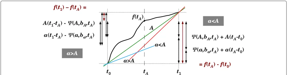
Figure 2Performance of the Four Point Method usingJCon K2P quartets with ti-tv ratioR=2.The concave non affine-additive SR

functionJCis shown (dashed green line) in the interval [t0,t1], wheret0andt1are the smallest and largest of the six pairwise distances (resp.). The dashed blue line shows the linear interpolationint=At+BofJCin the interval [t0,t1]. Horizontal dotted lines correspond to half of the two competing sums computed by FPM under the two SR functions (see legend).(a)In quartets of type A,t0=t12andt1=t34, and so

int(1, 2)+int(3, 4)=JC(1, 2)+JC(3, 4). However, fori∈ {1, 2}andj∈ {3, 4},int(i,j) < JC(i,j). Therefore, the deviation from additivity of

JCincreasesits FPM separation, denoted SEPJC, compared to the FPM separation SEPintofint.(b)In quartets of type B,t0=t13andt1=t24, and soint(1, 3)+int(2, 4)=JC(1, 3)+JC(2, 4). However,int(1, 2)=int(3, 4) < JC(1, 2)=JC(3, 4), and soint(1, 2)+int(3, 4) < JC(1, 2) +JC(3, 4). Therefore, the deviation from additivity ofJCdecreasesits FPM separation, denoted SEPJC, compared to the FPM separation SEPintof

int. Note that SEPintremains invariant in both types of quartets under fixedtiwhereas SEPJCchanges, depending on the type of quartet and the

ts/tlratio.

which provides a larger separation of the smallest sum from the two other sums will imply a better reconstruction probability.

We note that FC is not an exact indicator of the sep-arability in our case, because the necessary criteria for this are not satisfied in our model. Namely, the two dis-tance sums are not normally distributed, and they are correlated through the substitution process along the external edges of the quartet. Nevertheless, as Figure 3b suggests, FC turns out to provide a quite reliable com-parison of the expected performance of JC and K2P for the quartet series considered in the aforementioned experiment. Figure 3b exhibits for each quartet the FC of _JC alongside that of _K2P, both associated with the comparison of the true split (12|34) and the “_JC favored split” (13|24). As shown, the trends observed in both FC plots closely resemble the trends observed in the reconstruction accuracy plot (Figure 3a), and the the equilibrium point of the FC values of JC and

K2P is very close to the equilibrium point of the accu-racy of reconstructions of these two functions (near t_l/ts=3.6).

A useful feature of this framework is the natural way in which it teases apart the stochastic noise from the deviation from additivity. If we denote the numerator of FC by SEP (for “separation”) and its denominator by

NOISE, then a comparison of FC estimates between two SR function₁,₂can be represented as a ratio of ratios:

FC(1)

FC(2) =

SEP(1)

SEP(2)

/ NOISE(1) NOISE(2)

. (17)

Figure 4 illustrates how a comparison between the expected performance of_JCand that of_K2Pcan be car-ried out by tracing theSEPandNOISEratios along four series of homogeneous K2P quartet: the bottom-left plot corresponds to the quartet series considered in Figure 3; the plot above it corresponds to the same series with ti-tv ratioR=2; the two plots on the right describe two quar-tet series in which the weight of the short edges is constant ts=0.2, and the weight of the long edges ranges in [ 0.2, 1].

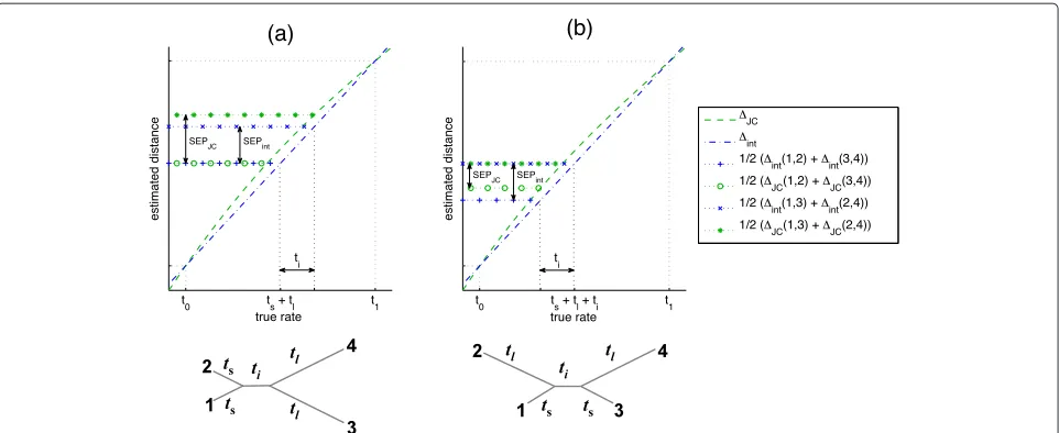
Figure 3Performance ofJCandK2Pon a series of quartets of type B.A series of homogeneous K2P quartets is considered (left illustration),

with ti-tv ratio ofR=5, and edge lengthsti=0.2,tl=1, andts∈[ 0.2, 1].(a)Reconstruction accuracy using FPM and eitherJC(dashed green) or

K2P(solid red) plotted againsttl/ts. Accuracy ratio is estimated using 100,000 independent replicates for each value oftsin the interval [ 0.2, 1] (in steps of 0.01), with sequence length 1,000 bp.(b)Fisher’s Criterion (FC) for the sums corresponding to splits(12|34)and(13|24)under eitherJC (dashed green) orK2P(solid red) plotted againsttl/ts.

theSEPratio, we see it becomes smaller (favoring_K2P) as the quartet becomes more unbalanced (theSEPratio decreases along the X axis in each of the four plots). This is because the deviation of_JCfrom additivity increases as the inter-leaf distance interval [t0,t1]=[t13,t24] expands. Deviation ofJCfrom additivity also increases with the ti-tv ratio, as the substitution model further departs from the assumptions of JC (theSEPratio forR=5 is consistently smaller than forR=2).

The two series on the right side of Figure 4 demon-strate well the tradeoff between the effects of stochastic noise and deviation from additivity. In both series, theSEP andNOISEratios decrease as the quartets become more unbalanced (due to the trends listed above). However, the rates of decrease of these two ratios are different due to the different ti-tv ratios, and this determines the expected relative performance of the two SR functions across the series. WhenR = 2, theSEPratio decreases at a slower rate than theNOISEratio, and_JCis expected to outper-form_K2Pacross the entire series. WhenR=5, theSEP ratio decreases at a faster rate than theNOISEratio, and when the quartets are sufficiently unbalanced (tl/ts > 4) K2Pis expected to outperformJC.

Simulations on Hasegawa’s Tree

In this section we describe experiments done on sim-ulated data sets generated along the seven-taxon tree

assembled by Hasegawa, Kishino, and Yano in 1985 [1,6]. This tree, spanning seven eutherian mammals (Figure 5a), was reconstructed originally using mitochondrial DNA sequences. It has a caterpillar topology (meaning that every internal node is incident to an external edge), and it has long external edges and short internal edges, making it a suitable representative of small phylogenetic trees spanning moderately distant species. These features also make it particularly challenging for distance-based reconstruction.

In our study we used the tree structure and edge lengths to generate simulated data sets. We considered the tree in various scales, by setting the tree diameter (largest inter-taxon path length) to values in the interval [ 0.1, 2.0]. For each scale considered, 10,000 simulations were carried out, where in each simulation 500 bp sequences were evolved along the tree according to a homogeneous K2P substitution model with ti-tv ratio ofR=2. For each sim-ulated data set, estimated values of the K2P statisticspα

andpβ, denoted bypˆα andpˆβ, were extracted for all

₇ 2

Figure 4SEPandNOISEratios.SEP(JC)/SEP(K2P)(dashed) andNOISE(JC)/NOISE(K2P)(dotted) plotted againsttl/tsfor four series of homogeneous K2P quartets of type B. Top two series have ti-tv ratio ofR=2, and bottom two series have ti-tv ratio ofR=5. Left two series have external edge lengthstl=1 andts∈[ 0.2, 1], and right two series have external edge lengthstl∈[ 0.2, 1] andts=0.2. The length of the internal edge is constantti=0.2 in all four series.

Sequence simulation was performed using SeqGen [34] (by choosing the HKY model with uniform base frequen-cies), and tree reconstruction was performed using the version of NJ implemented in the PHYLIP package [35].

We studied the reconstruction accuracy associated with four different SR functions:JC,K2P,tv, andR=2. The first two are as described in Equations (5) and (4), respec-tively. The third SR function,tv, considers only tv-type substitutions:tv(pα,pβ) = −1₄log

1−4pβ(t)

= βt, and the fourth SR function, R=2, is based on a max-imum likelihood (ML) estimatorg _{of the time t from} the estimated transition probabilities pˆα,pˆβ, given that

R = 2. Informally, this function, which uses knowledge of the true value of R (which is typically unknown to the user), is optimal in our setting, because it has sim-ilar stochastic noise as _JC, and it is additive since it coincides with _K2P when applied to transition prob-abilities pˆα,pˆβ that are consistent with a ti-tv ratio of

R=2.

The performance of these four SR functions is traced across the different tree scales in Figure 5a. For each SR functionand scales, we recorded the average normal-ized RF distance from the true tree to each of the 10,000 trees reconstructed using . The RF distance was nor-malized by its maximum value which is twice the number of internal edges in the tree (in our case 2× 4 = 8). As observed previously in [9], K2P performed well in shorter scales, andtv performed well in longer scales. However, both additive SR functions were significantly outperformed in nearly all cases byJC. Surprisingly,JC even slightly outperformedR=2. We speculate that this happened due to a bias similar to the one observed in type A quartets in Section Performance of Non affine-additive SR Functions in Quartet Resolution, improving the performance of concave SR functions such as_JCon certain K2P-trees.

Figure 5Simulations on Hasegawa’s Tree.(a)Reconstruction accuracy of four different SR functions on different scaled versions of Hasegawa’s tree [6]. The tree with scaled edge weights is depicted (left) next to the graph (right) plotting reconstruction accuracy of four SR functions. Different scales of the tree are considered, indicated by the diameter of the tree (X axis). Reconstruction accuracy (Y axis) is measured for each scaled tree by the average normalized RF distance between the reconstructed tree and the true tree across 10,000 simulated data sets. Simulations were carried out assuming a ti=tv ratio ofR=2 and sequence length of 500 bp.(b)A similar plot is shown for a semi-symmetric caterpillar tree.

with internal edges of uniform length tint, and external

edges of uniform lengthtext =5tint(Figure 5b). The

sym-metry of this tree was expected to reduce the effect of the reconstruction bias observed in Hasegawa’s tree, and indeed, _JC performed much more poorly on this tree. Despite this fact,JCstill outperformedK2Pin all scales andtvin the smaller scales (s<1.1).

Inferring trees from genomic sequences

In this section we describe our study comparing various SR functions on genomic DNA sequences. Next to JC andK2P we also considered the well known LogDet SR function [36,37], denoted here asLogDet. Extending our study to this setting is challenging in two respects. First of all, unlike the simulated case, the true tree is not known with complete confidence, and accuracy of reconstruction can only be determined by using a well-accepted refer-ence tree that may contain some errors. Secondly, the true substitution model is also unknown and is likely to vio-late the assumptions of both JC and K2P models and even

the relaxed assumptions of the general time-reversible model (in which_LogDet is additive). Hence, we have to assume in this case that _JC, _K2P, and _LogDet are all non affine-additive, where _JC and_K2P are still likely to exhibit higher deviation from additivity than_LogDet, since they make stronger assumptions on the substitution model.

The genomic data set

and found 199 bacterial genomes that contained all anno-tated COGs. For each of the 31 COGs, we extracted the appropriate protein sequence in each of the 199 bacterial species, choosing an arbitrary paralog in cases of multiple hits. We followed a procedure similar to the one described in [38,39] to obtain reliable multiple-sequence alignments for each COG: we computed a 199-way multiple align-ment of the protein sequences of each COG using HMMa-lign [40] and then mapped each protein sequence back to its coding DNA sequence. The conserved parts of each of the 31 DNA alignments were extracted using GBLOCKS [41] to filter out alignment columns with 50% or more gap symbols. The alignments were manually scanned, and 36 species which contributed a large number of gaps to the alignments were removed from the subsequent analysis. The 31 different alignments were concatenated to form one long 163-way multiple sequence DNA alignment.

For the reference tree we used the phylogenetic tree of microbial species provided by the ARB-SILVA Living Tree Project [42]. This tree, spanning 8,029 species at the time of writing, is based on a widely accepted analysis of the small subunit (SSU) 16S RNA. A subtree spanning our 163 bacterial species was extracted from this tree and treated as the true phylogenetic tree in our analysis.

Reconstruction accuracy for ten-species subsets

We used the base set of 163 species to generate 40,000 random 10-species sub-alignments. The random selection process was guided to generate species subsets corre-sponding to a wide range of diameter scales (a blind random selection process is biased toward subsets with large diameters). For each of the 40,000 subsets, a 10-way subalignment was extracted from the original 163-way alignment, and in this alignment we extracted only columns corresponding to four-fold degenerate sites that do not have any gap symbol. This is done to make sure the sites used for distance estimation have undergone a substitution process that is as uniform as possible along the different lineages and across the different sites. Each sub-alignment was used to compute three distance matri-ces – one under _JC, one under _K2P, and one under _LogDet. The latter was calculated by the version that is implemented in the PHYLIP package. The NJ algorithm was then applied to the three matrices and the resulting trees were compared to the true tree (as depicted by the appropriate LTP subtree) according to the RF distance.

As an additional comparison, we used a fourth recon-struction technique. This method (termed BIONJ-GTR) used the BIONJ reconstruction algorithm [43] on dis-tances obtained under the general time-reversible model with invariant sites and Gamma distribution of rates across variant sites (GTR++I) [8,44].

The PhyML package [45] was used to infer this tree for each of the 40,000 subsets. We selected the GTR++I

model since it was found by the MEGA5 software [46] to provide the best fit to the sequence data. The 40,000 sampled instances were partitioned into eight bins accord-ing to the RF distance observed between the BIONJ-GTR tree and the true (LTP) tree, and average RF distances were recorded for each of the three SR functions in each bin. This allowed us to observe trends throughout these 40,000 samples (Figure 6). Of the 40, 000 trees inferred under_JC, 83.1% showed an equal or lower RF distance than those reconstructed by the BIONJ-GTR method. Moreover,_JCoutperformed_K2Pand_LogDeton aver-age in all partitions, and_LogDetshowed by far the worst performance with 48.7% of all reconstructed trees achiev-ing higher RF distances to the reference tree than those inferred by BIONJ-GTR. As with our results on simulated data sets, we see that the SR functions with lower stochas-tic error but inferior model fit performed best. Unsur-prisingly, the GTR+G+I model itself, which was predicted to have the best fit to the sequence data, was often out-performed by the simpler JC and K2P models. Note that the difference in performance betweenJC and the two other SR functions is greater for subsets that are more accurately reconstructed by the BIONJ-GTR approach (the lower bins). This appears to indicate that over-simplified distance methods are particularly beneficial when the sequence data conveys a stronger phylogenetic signal.

Conclusions

Figure 6Evaluation against BIONJ-GTR tree.The 40,000 subsets of size 10 were partitioned according to the the RF-distance between the reference LTP tree and the tree reconstructed using BIONJ-GTR (X axis). The (left) Y axis describes the mean difference between the RF-distance associated with a tree reconstructed using a particular SR function (K2P,JC, orLogDet) and the RF-distance associated with the BIONJ-GTR tree. The bar plot in the background depicts the number of subsets in each bin.

homogeneous K2P-tree with an unknown ti-tv ratioR. In this case, Kimura’s distance formula_K2Pis always addi-tive, while the less noisy Jukes Cantor’s formula,_JC, is additive only whenR= 1₂.

A study of this type requires a way to measure the deviation from additivity of a non-additive SR function in a given range of distances [t0,t1]. To this end, we introduced the concept of affine-additive distance func-tions, and defined the deviation from additivity of in [t0,t1] as the distance of from its closest affine-additive function in [t0,t1]. We established a tight con-nection between this measure and statistical consistency of reconstruction (Lemma 2.7) and derived an upper bound for deviation from additivity in homogeneous models (Lemma 2.8). We applied these results in analyz-ing the deviation from additivity of_JC, and its effect on the accuracy of reconstructing homogeneous K2P-trees.

We then showed, both analytically (in Section Devia-tion from Additivity in Homogeneous SubstituDevia-tion Mod-els) and through experiments on simulated data sets (in Sections Performance of Non affine-additive SR Functions in Quartet Resolution and Simulations on Hasegawa’s Tree), that, compared to K2P, it is often better to use the non-additive but less noisy estimates of JC, even when R is quite high. Somewhat surprisingly, we found this to be the case even when the tree being recon-structed has an “unfavorable” topology. Our experiments on bacterial gene sequences (Section Inferring Trees from Genomic Sequences) also indicate that the simple and less noisy SR functions perform better on average than ones that are expected to better fit the true substitution process.

The framework presented in this paper implies a prac-tical way for selecting SR functions which are likely to

increase the accuracy of distance estimation. The practi-cality of the method is drawn from the fact that the criteria by which we select an SR function depend only a relatively crude information about the tree being reconstructed. For instance, in the case of a homogeneous K2P-tree, one can easily obtain from the input sequences rough esti-mates of both the ti-tv ratioRand the range of inter-leaf times [t0,t1]. These estimates can then be used to com-pare the expected accuracies of_JCand_K2Pon the given input, and determine which of them is more likely to yield an accurate phylogeny. For quartets, a tight comparison can be made using the FC-based approach suggested in Section Fisher’s Criterion for Separability, and for larger trees, a cruder comparison can be made using a plot like the one presented in Figure 1b. A promising avenue of further research is to extend the FC-based approach to allow tighter prediction of reconstruction accuracy of trees spanning more than four taxa.

Endnotes

a_{This is a WABI 2011 special issue invited paper. Extended}

abstract of this paper appeared in [47].

b_{Typically, the unit rate matrix is assumed to be the one}

corresponding to one substitution per site.

c_{Many common distance-based algorithms, such as the}

Neighbor Joining (NJ) algorithm [31,32], are known to be robust in this sense.

d_{In a tree, edges which touch leaves areexternal, and all}

other edges areinternal.

e_{Types A and B quartets represent the Farris zone and}

Felsenstein zone, resp. (see, e.g., [1], Chapter 9).

f_{We use here the square root of the criterion commonly}

used in the literature, because we prefer to think in terms of distances rather than squares of distances. This has no practical influence, since we use FC only for comparing between different choices, not for assessing the quality of a give choice.

g_{This ML estimate is obtained by a simple numerical}

method for maximizing the likelihood function (see, e.g., [1]).

Appendix

Tightness of Lemma 2.8.

Let f(t) be a (continuous) function on some interval [t0,t1]. We prove below that if f does not intersect its linear interpolation At + B in that interval, then dev(f, [t0,t1]) = _A1maxt∈[t0,t1]

|f(t)−At−b∗|. We use the following notations, conforming to the notations in the proof of Lemma 2.8:

ψ (a,b,t) = f(t)−at−b ψ (a,b)= max

t∈[t0,t1]{|

ψ (a,b,t)|} ψ (a)=min

b∈R{ψ (a,b)}.

Lemma 2.9.Let f(t)be a monotone increasing function in the interval[t0,t1]and let At+B be its linear

interpo-lation in[t0,t1]. If either f(t)≥At+B for all t∈[t0,t1]or

f(t)≤At+B for all t∈[t0,t1], then for all a>0, we have 1

aψ (a) ≥ A1ψ (A).

Proof.We prove the minimality of _A1ψ (A) in the case where f(t) ≥ At+ Bfor all t ∈[t0,t1]. The other case (wheref(t) ≤At+Bfor allt∈[t0,t1]) can be proven in an identical fashion.

For a > 0, let ba be the maximum value of b s.t. ψ (a,b,t) ≥ 0 for all t ∈[t0,t1]. Evidently, ψ (a) =

1

2ψ (a,ba). If the linear interpolation off(t)in [t0,t1] is given byAt+B, thenbA = B. We need to show that for

everya > 0, it holds thatAψ (a,ba) > aψ (A,bA). LettA

be a point in [t0,t1] s.t.ψ (A,bA,tA)=ψ (A,bA). Note that

ifa<A, then the two linear functionsAt+bAandat+ba

intersect at(t0,f(t0)), and ifa>A, then they intersect at

(t1,f(t1))(see Figure 7).

Fora<A, we get the following equality (Figure 7; right):

ψ (A,bA,tA)+A(tA−t0) = f(tA)

−f(t0) = ψ (a,ba,tA)+a(tA−t0). (18)

Hence, sinceψ (a,ba)≥ψ (a,ba,t)for everyt∈[t0,t1], and sincea<A, we get

aψ (A,bA,tA)+aA(tA−t0) < Aψ (a,ba,tA)

+Aa(tA−t0)⇒ aψ (A,bA) <Aψ (a,ba).

Similarly, if a > A, we get the following equality (Figure 7; left)

A(t1−tA)−ψ (A,bA,tA) = f(t1)

−f(tA) = a(t1−tA)−ψ (a,ba,tA),

(19)

anda>Aimplies that

aA(t1−tA)−aψ (A,bA) >Aa(t1−tA)

−aψ (a,ba) ⇒ aψ (A,bA) <Aψ (a,ba).

Competing interests

The authors declare that they have no competing interests.

Authors’ contributions

All authors participated in discussing, formulating, and modulating the research. DD performed the simulations and experiments of Sections Simulations on Hasegawa’s Tree and Section Inferring Trees from Genomic Sequences. IG and SM initiated and directed the research and drafted the manuscript. IY performed the analysis in Sections Deviation from Additivity in Homogeneous Substitution Models and Section Performance of Non affine-additive SR Functions in Quartet Resolution and contributed to the ideas of the project. All authors contributed to the writing and editing of the manuscript, and all authors read and approved the final manuscript.

Acknowledgements