S O F T W A R E A R T I C L E
Open Access
gammaMAXT: a fast multiple-testing
correction algorithm
François Van Lishout
1,2*, Francesco Gadaleta
1,2, Jason H. Moore
3, Louis Wehenkel
1,2and Kristel Van Steen
1,2*Correspondence: [email protected] 1Systems and Modeling Unit, Montefiore Institute, University of Liège, Allée de la découverte 10, 4000 Liège, Belgium
2Bioinformatics and Modeling, GIGA-R, Avenue de l’Hôpital 1, 4000 Sart-Tilman, Belgium
Full list of author information is available at the end of the article
Abstract
Background: The purpose of the MaxT algorithm is to provide a significance test algorithm that controls the family-wise error rate (FWER) during simultaneous hypothesis testing. However, the requirements in terms of computing time and memory of this procedure are proportional to the number of investigated hypotheses. The memory issue has been solved in 2013 by Van Lishout’s implementation of MaxT, which makes the memory usage independent from the size of the dataset. This algorithm is implemented inMBMDR-3.0.3, a software that is able to identify genetic interactions, for a variety of SNP-SNP based epistasis models effectively. On the other hand, that implementation turned out to be less suitable for genome-wide interaction analysis studies, due to the prohibitive computational burden.
Results: In this work we introduce gammaMAXT, a novel implementation of the maxT algorithm for multiple testing correction. The algorithm was implemented in software MBMDR-4.2.2, as part of the MB-MDR framework to screen for SNP-SNP,
SNP-environment or SNP-SNP-environment interactions at a genome-wide level. We show that, in the absence of interaction effects, test-statistics produced by the MB-MDR methodology follow a mixture distribution with a point mass at zero and a shifted gamma distribution for the top 10 % of the strictly positive values. We show that the gammaMAXT algorithm has a power comparable to MaxT and maintains FWER, but requires less computational resources and time. We analyze a dataset composed of 106 SNPs and 1000 individuals within one day on a 256-core computer cluster. The same analysis would take about 104times longer withMBMDR-3.0.3.
Conclusions: These results are promising for future GWAIs. However, the proposed gammaMAXT algorithm offers a general significance assessment and multiple testing approach, applicable to any context that requires performing hundreds of thousands of tests. It offers new perspectives for fast and efficient permutation-based significance assessment in large-scale (integrated) omics studies.
Keywords: Multiple testing, Genome-wide interaction studies, MaxT, Gamma distribution, SNP-environment interactions, 3-order interactions, Algorithmic
Background
Personalized medicine proposes to customize healthcare using molecular analysis [1–5]. However, for most human complex diseases, a deeper comprehension of the under-lying biology is needed to make this approach workable. Since individual genes usually do not account for much of the heritability of phenotypes, the focus should be on the combined effect of all the genes in the background, rather than on the disease genes
in the foreground [6–9].MBMDR-4.2.2 is a software dedicated to genome-wide asso-ciation interaction studies (GWAIs), the purpose of which is to identify pairs of SNPs and/or environmental factors that might regulate the susceptibility to the disease under investigation. The difficulty is to find a good balance between four main issues, that we summarise in the following objectives:
(1) Minimize the amount of false discoveries.
(2) Achieve sufficient statistical power to detect relevant pairs.
(3) Reduce the computational burden implied by the high number of tests for
interactions.
(4) Provide a versatile software package that accommodates different study designs
and study features, including flexibility in trait measurement types and the possibility to adjust for important predictor variables and confounders.
Available software
(1), (2) and (4) [22, 23]. However, concerns about computational efficiency remain when scaling up to exhaustive genome-wide interaction contexts. In this work we introduce a new version of the software,MDMDR-4.2.2, based on a novel multiple-testing correction algorithm, with the purpose of improving the performances along objective (3), with the same benefits as before regarding the other three ones.
Multiple-testing correction
In GWAIs, the most global null hypothesis is that none of the SNPs pairs, nor their main effects, are associated with the trait. Testing each pair independently at level α does not control the overall FWER at level α; an adjustment is needed for the fact that multiple tests are performed. One such adjustment can be realized via a Bonfer-roni correction [24]. This is a so called single-step procedure for strong FWER control. Single-step methods tend to be conservative though and improvements in power can be achieved by so called step-down procedures [25]. Among these we recall step down minP adjustedp-values (minP) and step down maxT adjustedp-values (maxT). These methods guarantee strong control of the FWER under the subset pivotality assumption and weak control under all conditions [26]. Both procedures are available in MDMDR-3.0.3, the adjusted p-values being estimated by permutation. Since a high number of pairs of SNPs are tested, minP tends to be more conservative than maxT [25]. Fur-thermore, minP requires more computations than maxT. For these reasons, maxT is the default choice in MDMDR-3.0.3. Note that the drawback of maxT compared to minP, is that when the test statistics are not identically distributed unbalanced adjust-ments can be observed because not all tests contribute equally to the computed adjusted p-values.
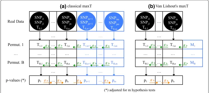
Figure 1(a) describes the classical implementation of maxT in MB-MDR. Test-statistics are computed for allmpairs of SNPs and sorted in decreasing order in vectorReal Data. The trait is permutedBtimes and test-statistics are computed for all pairs of SNPs and stored in vectorsPermutationi,i=1,. . .,B. The latter are browsed from right to left and any value higher than its left neighbor’s value overwrites the latter value. This step is an
Fig. 1classical MaxT versus Van Lishout’s implementation of MaxT. In the classical implementation of MaxT, allTi,jvalues are computed and stored in memory,∀i=0. . .B,∀j=1. . .m. Then,Ti,jis overwritten byTi,j+1 wheneverTi,j+1>Ti,j,∀i=1. . .B,∀j=m−1. . .1. Finally,pj+1is overwritten bypjwheneverpj>pj+1,
algorithmic trick to reach efficiently an idea that is best explained the other way around. LetTi,maxbe the maximum ofPermutationi,i= 1,. . .,B. TheTi,maxvalues can be used to approximate the distribution of the highest observed value when testingmpairs under the global null hypothesis (no pair of SNPs associated to the disease). ComparingT0,1 to this distribution enables the computation of adjustedp-valuep1, i.e. the probability of observing a value as extreme asT0,1for the most promising pair of SNPs. Removing the latter from the data and restarting the whole procedure would obviously allow the computation of adjustedp-valuep2and so on for the remaining ones. From an algorith-mic point of view, this would be a waste of time, hence the aforementioned procedure leading to the same result. Finally, the adjustedp-values are browsed from left to right and any value higher than its right neighbors’s value overwrites the latter. This procedure obviously aims at controlling the FWER. A particular hypothesis can indeed now only be rejected if all hypotheses were rejected beforehand. The problem of the original maxT is that it is both time and memory consuming.
Van Lishout’s implementation of maxT solves the latter issue [23]. It is based on the observation that in practice, only a few adjusted p-values will point towards interest-ing interactions to investigate. With this in mind, it adapts the original method such that it still calculates the test-statistics of all pairs, but only computes the adjusted p-values of the n best pairs, i.e. the ones with the n lowest adjusted p-values. The default value isn = 1000 and can be tuned without loss of generality according to the researcher’s needs. Note that despite the fact that onlynadjustedp-values are produced, they are still adjusted at the overall level, i.e. for the m association tests. Figure 1(b) describes Van Lishout’s MaxT implementation. The different steps are reported in Table 1.
Bottlenecks of Van Lishout’s maxT
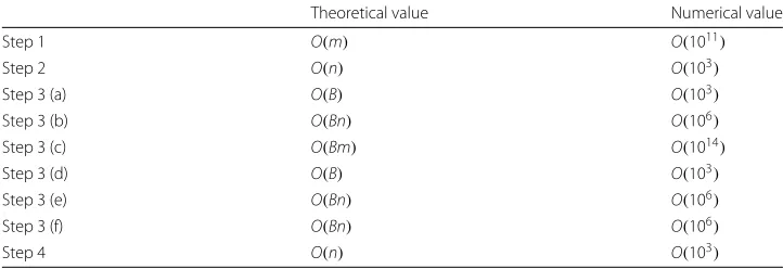
Van Lishout’s implementation of maxT still leaves room for improvement. In what fol-lows, we identify its main bottlenecks, in order to improve the overall performance on large-scale data. In Table 2 we report the number of operations performed (with the default parameters of the softwaren = 1000 andB= 999) on a dataset containing 106 SNPs, which is equivalent tom≈5×10¹¹pairs of SNPs.
Table 2 reflects that in step 1 of Van Lishout’s maxT, as many elementary compu-tations are carried out as there are SNP pairs to test. Although significance assess-ment can be based on fewer SNP pairs, this first step of computing test values
Table 1Van Lishout’s MaxT
(1) Compute the test-statistics for all pairs, but only store thenhighest tests values. The result is aReal data vector whereT0,1≥T0,2≥. . .≥T0,n.
(2) Initialise a vectorpof sizenwith 1’s.
(3) Perform the following operations fori=1,. . .,B: (a) Generate a random permutation of the trait column. (b) ComputeTi,1,. . .,Ti,nand store them in aPermutationivector. (c) Compute the maximumMiof the test-statistics valuesTi,n+1,. . .,Ti,m. (d) ReplaceTi,nbyMiifTi,n<Mi.
(e) Force the monotonicity of thePermutationivector: forj=n−1,. . ., 1 replaceTi,jbyTi,j+1ifTi,j<Ti,j+1. (f) For eachj=1,. . .,n, ifTi,j≥T0,jincrementpjby one.
Table 2Analysis of the computing times of the different steps of Van Lishout’s implementation of MaxT on a dataset containing 1 million SNPs
Theoretical value Numerical value
Step 1 O(m) O(1011)
Step 2 O(n) O(103)
Step 3 (a) O(B) O(103)
Step 3 (b) O(Bn) O(106)
Step 3 (c) O(Bm) O(1014)
Step 3 (d) O(B) O(103)
Step 3 (e) O(Bn) O(106)
Step 3 (f) O(Bn) O(106)
Step 4 O(n) O(103)
and ordering them cannot be avoided nor simplified. However, the most computa-tionally intensive part of the significance assessment procedure is step 3(c). With 106 inputted SNPs, the number of elementary computations required is proportional to 1014. Therefore, any improvement at this stage will lead to better overall per-formances. In “Methods” section, we introduce a novel algorithm for multiple test-ing, based on Van Lishout’s implementation of maxT. It is implemented in the
software MBMDR-4.2.2 and resolves remaining concerns about maxT’s
computa-tion time in genome-wide screens for genetic interaccomputa-tions using the MB-MDR framework.
Methods
In MBMDR-4.2.2 the value of Mi from Fig. 1 will be estimated from a sample from [Ti,n+1,. . .,Ti,m] rather than calculated exactly. A detailed explanation of how we perform such an improvement is provided in the next section.
Distribution of MB-MDR statistics
interaction study, those subjects having two copies of the minor allele at each locus) is compared to the remaining subjects with respect to the trait under study and by using an appropriate association test statistic, this group can either be associated to a higher “risk” (“H” category), a lower “risk” (“L” category) or undecisive “risk” (nor “H”, nor “L”; “O” cate-gory) for the trait. Here, “risk” is used loosely. For instance for continuous traits, the “risk” categories above may rather refer to increased (“H” category), decreased (“L” category) mean trait values. Also, in the MB-MDR methodology, risk scales can be refined to incor-porate multiple risk categories. It is important to realize that if all subjects are assigned the same label (in this scenario, most probably the “O” label), then MB-MDR will return an exact zero. It is not surprising that lack of power of GWAIs (which depends on sample size but also true effect size) will induce such technical zeros for a significant proportion of the tested SNP pairs. In order to take this important amount of zeros into account, we use the approach described in [31]. We assign a discrete probability mass to the exact zero value. Hence, ifXiis a random variable returning a random value from [Ti,n+1,. . .,Ti,m], withi > 0, we can define the probabilitiesπ = P(Xi > 0)and 1−π = P(Xi = 0). Therefore, the distribution ofXi is semi-continuous with a discontinuity at zero. This implies that the probability density function isfXi(x) = (1− π)δ(x)+πgXi(x)1(x>0), whereδ(x)is a point probability mass atx = 0,gXi(x)is the distribution of the strictly positive values and1(x>0)is an indicator function taking the value 1 ifx> 0 and 0 oth-erwise. The parameterπ depends on the data at hand and can be estimated with the Maximum Likelihood Estimation (MLE) method [32] from the observed frequency in a sample from [Ti,n+1,. . .,Ti,m]. Due to the fact that our main goal consists in predict-ing a maximum, we are not particularly interested in fittpredict-ing the distribution ofgXi(x) on the entire set of strictly positive values. As a matter of fact, fitting the tail ofgXi(x) should suffice. We show in the next section that focusing on the top 10 % strictly pos-itive values is an acceptable practical choice. We consider this a good tradeoff between fitting on a large and a smaller range of positive values. The former might lead to a poor fit of the tail, because many samples might not belong to that range. The latter might lead to a poor fit of the tail due to an insufficient number of samples. The amount of values belonging to the top 10 % strictly positive values in [Ti,n+1,. . .,Ti,m] is given by
q= (m−10n)π.
Assumption 1
We assume that the shifted gamma distribution is a good fit to the tail ofgXi(x). Hence, ifYiis a random variable returning a value from the aforementioned top 10 % of strictly positive values, we postulate that its cumulative distribution function (CDF) is given by
FYi(y) = γk,y−y0
θ
Table 3Mean and variance of the fitted parameters for datasetsD1−D4
D1 D1 D2 D2 D3 D3 D4 D4
Mean Var Mean Var Mean Var Mean Var
π 0.337 1.247×10⁻⁶ 0.335 3.815×10⁻⁶ 0.137 4.948×10⁻⁷ 0.366 9.356×10⁻⁷
y0 7.742 5.566×10⁻⁴ 7.825 8.778×10⁻⁴ 6.189 6.472×10⁻⁴ 7.788 3.805×10⁻⁴
k 1.017 2.612×10⁻⁴ 1.012 2.534×10⁻⁴ 0.990 3.580×10⁻⁴ 1.017 1.725×10⁻⁴
θ 1.917 1.462×10⁻³ 1.974 1.532×10⁻³ 1.694 1.829×10⁻³ 1.917 9.695×10⁻⁴
positive value should not be in the neighborhood of zero. Indeed, a small value would represent a low-significant association between the interaction of the two loci and the phenotype. As previously mentioned, this would lead to the “O” category for all subjects and an exact zero. The CDF of the random variableZi returning the maximum of the
qvalues belonging to the top 10 % strictly positive values in [Ti,n+1,. . .,Ti,m] is given by
FZi(z)=
γk,z−y0 θ
(k)
q
. Indeed, if we takeqindependent and identically distributed (i.i.d.)
valuesy1,y2,. . .,yq, thenP[(y1≤yt)∧(y2≤yt)∧. . .∧(yq≤yt)]=[FYi(yt)]q=FZi(z).
Assumption 2
We postulate that the parameters π, y0, k andθ are stable from one permutation to another. This assumption is a plausible one, given the results in Table 3, which show low variance of these parameters across 999 permutations. An analogous observation has been noticed in a similar work [34], based on hypothesis testing with an extreme value distribution. In order to reduce the computational burden of the fitting, we estimate the parameters once every 20 permutations. We consider this a compromise between robustness and performance.
Estimating the parameters of the shifted gamma distribution
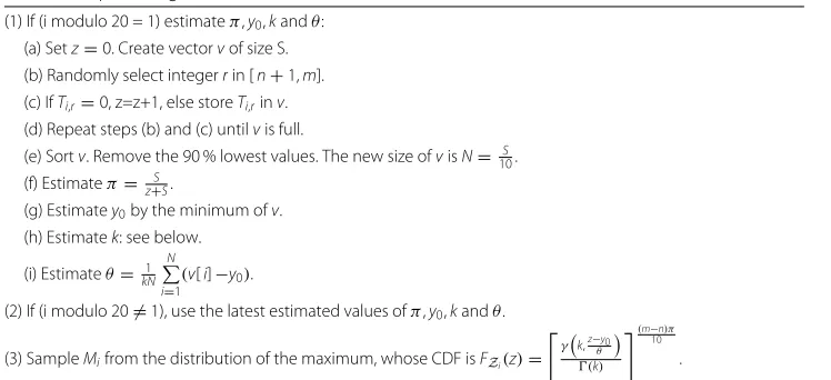
As mentioned in the introduction, the gammaMAXT algorithm only differs from Van Lishout’s implementation of maxT (Table 1) with respect to step 3(c). In the novel imple-mentation the maximum Mi is estimated from a sample of size S = 106 of strictly positives values in [Ti,n+1,. . .,Ti,m] rather than calculated directly. The parameterπ is
Table 4Step 3(c) of gammaMAXT
(1) If (i modulo 20 = 1) estimateπ,y0,kandθ: (a) Setz=0. Create vectorvof size S. (b) Randomly select integerrin [n+1,m]. (c) IfTi,r=0, z=z+1, else storeTi,rinv. (d) Repeat steps (b) and (c) untilvis full.
(e) Sortv. Remove the 90 % lowest values. The new size ofvisN= 10S. (f) Estimateπ=z+SS.
(g) Estimatey0by the minimum ofv. (h) Estimatek: see below.
(i) Estimateθ= kN1 N
i=1( v[i]−y0).
(2) If (i modulo 20=1), use the latest estimated values ofπ,y0,kandθ. (3) SampleMifrom the distribution of the maximum, whose CDF isFZi(z)=
γk,z−y0
θ
(k) (m−n)π
estimated on the fly using a variablez, counting the amount of zeros encountered during the sampling process. The new step 3(c) is described in Table 4.
Whereas estimates in steps (1)(f ), (1)(g) and (1)(i) are obtained via Maximum Like-lihood, the estimation of the parameter k requires more elaboration. According to [35], an acceptable initial guess being within 1,5 % of the correct value is given by
k = 3−s+ √
(s−3)2+24s
12s , with s = ln
1 N
N
i=1(
v[i]−y0)
− 1 N
N
i=1
ln(v[i]−y0). This
ini-tial guess is updated iteratively via the Newton-Raphson method [36]. In particular, in every iteration, k is updated as k = k− ln(k)1−ψ(k)−s
k−ψ(k)
until the difference between
the new and the old value ofk is lower than the desired precision (default: 0.000001).
ψ(k)andψ(k)are respectively the digamma and trigamma functions. Finally, Table 5 describes the procedure used at step (3) to compute the finalMi estimation. Note that we have to sample and not take the expectation, in order to mimic the original maxT algorithm.
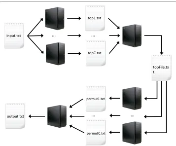
Parallel workflow
Figure 2 describes the four steps of the parallel workflow developed to further make MBMDR-4.2.2suitable for GWAIs. The detailed algorithm is given in Table 6.
Results and discussion
In this section, we first show results supporting the two assumptions on which the novel algorithm is based. Then, we analyse the performances in terms of computing-time, power and control of the FWER.
Results supporting assumption 1
In this part, we investigate the hypothesis that the tail ofgXi(x)follows a shifted gamma distribution and that fitting the top 10 % of strictly positive values is an acceptable choice. We use the following datasets for this experiment:
• A simulated datasetD1expressed on a binary scale, composed of 1000 SNPs and
1000 individuals. Table 7 states the two-locus penetrance table used to generate it. A balanced number of cases and controls is sampled. The minor allele frequencies of the functional SNPs are fixed at 0.5 and those of the non-functional SNPs are randomly generated from a uniform distribution on [0.05, 0.5]. This corresponds to the first of six purely epistatic models discussed in [15]. Furthermore, any value in the dataset had a 5 % chance to be missing.
• A simulated datasetD2, with the same properties asD1, except that the trait is
expressed on a continuous scale.
• A simulated datasetD3, with the same properties asD1, except that the MAF’s are on
average lower, i.e. the non-functional SNPs were randomly generated from a uniform distribution on [0.05, 0.1].
Table 5SampleMiwhen CDF isFZi(z)
(a) Take a too high initial guess ofMi(default: 1000). Initialize variablebto half of this value. (a) Randomly select a real numberrn∈[0, 1].
Fig. 2MBMDR-4.2.2parallel workflow. First, each cluster node performs a fair proportion of theT0,1,. . .,T0,m values from Fig. 1 and saves thenhighest into filetop_c.txt. Second, a node aggregates alltop_c.txtfiles and retrieves the overallnhighest values, saved intopfile.txt. Third, each cluster node readstopfile.txtand performs an equitable fraction of theBpermutations of Fig. 1, saving results into filepermut_c.txt. Finally, a cluster node aggregates allpermut_c.txtand produces the final output file
• A real-life datasetD4on Crohn’s disease, for which the trait is expressed on a binary
scale [37, 38], reduced to 12471 SNPs and 1687 subjects as in [23].
For each of the aforementioned datasets, we first carry out the initial Van Lishout’s implementation of maxT based on 104permutations to generate a reference distribution
Table 6gammaMAXT parallel workflow
(1) Each cluster nodec=1. . .Cperforms an equitable fraction of the computations of theT0,1,. . .,T0,m values from Fig. 1. Thenhighest values (and corresponding SNP pair indexes) from each node are saved into filetop_c.txt.
(2) Upon termination of all computations at the previous step, a cluster node aggregates alltop_c.txtfiles and retrieves the overallnhighest values (and corresponding SNP pair indexes). Results are saved intotopfile.txt. (3) Each cluster node readstopfile.txt, initialize a vectorVof sizenwith 0’s and performs an equitable fraction
of theBpermutations of Fig. 1. For each permutationiattributed to nodec: (a) Generate a random permutation of the trait column.
(b) ComputeTi,1,. . .,Ti,nand store them in aPermutationivector. (c) Execute step (3)(c) of the gammaMAXT algorithm to estimateMi. (d) ReplaceTi,nbyMiifTi,n<Mi.
(e) Force the monotonicity of thePermutationivector: forj=n−1,. . ., 1 replaceTi,jbyTi,j+1ifTi,j<Ti,j+1. (f) For eachj=1,. . .,n, ifTi,j≥T0,jincrementVjby one.
Upon completion of all computations on nodec, saveVinto filepermut_c.txt.
Table 7Two-locus penetrance table used to create the simulated datasetsD1,D2andD3
b/b b/B B/B
a/a 0 0.1 0
a/A 0.1 0 0.1
A/A 0 0.1 0
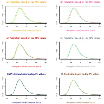
for Mi. We second execute step (3)(c) of the gammaMAXT algorithm based on 104 permutations, with different values for the internal parameter defining the percentage of strictly positive values belonging to the tail ofgXi(x). Figure 3 is generated in R and shows the results for datasetD1. We observe that focusing on respectively 25, 20, 15, 5 and 1 % of the strictly positive values leads to a good fit, but that 10 % is the optimal alternative. The curves of subfigure (d) are indeed close and the Kolmogorov-Smirnov (KS) distance is the lowest among these choices. This supports the hypothesis that the gammaMAXT algorithm produces accurate predictions of theMi values. Addditional file 1: Figure S1, Addditional file 2: Figure S2 and Addditional file 3: Figure S3 show that 10 % is consistently a good option, although not always the most optimal one.
Results supporting assumption 2
In this section, we show results supporting the hypothesis that parametersπ,y0,kand
θ are stable across permutations. We perform MBMDR-4.2.2 analyses on datasetsD1 to D4, using the default settings. For this experiment, we modified the gammaMAXT algorithm such that it fits new parameters for each of the 999 permutations (not only once every 20 as previously mentioned) and saves these into a file. We report their means and variances in Table 3. We observe that the variance is very low across all scenarios.
Computing-time of the gammaMAXT algorithm
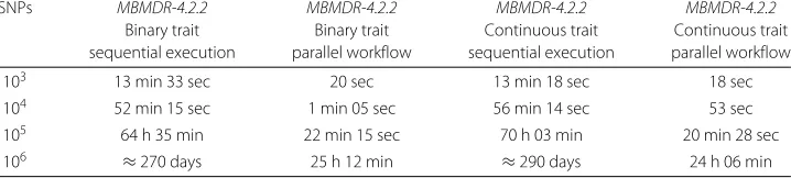
In order to assess the speed performances of MBMDR-4.2.2, we created 4 different datasets with 1000 individuals each, of respectively 103, 104, 105 and 106 SNPs. All datasets were generated using GAMETES, a fast, direct algorithm for generating pure epistatic models with random architectures [39]. Another set of 4 datasets, containing the same number of individuals and SNPs, but expressing the trait on a continuous scale, was created using a similar strategy as forD2. The parallel workflow ofMBMDR-4.2.2 has been tested on a 256-core computer cluster (Intel L5420 2.5 GHz). The sequential version has been tested on a single core of this cluster. Table 8 shows the results. We observe thatMBMDR-4.2.2outperforms the computing times ofMBMDR-3.0.3reported in [23]. For instance, solving a continuous dataset of 104SNPs on a single core takes about 56 min withMBMDR-4.2.2and almost 12 days withMBMDR-3.0.3, i.e. about 300 times less. Solving a continuous dataset of 106SNPs on a 256-core cluster takes about one day withMBMDR-4.2.2and would take about 104longer withMBMDR-3.0.3. In general, the theoretical computing time of step 3 (c), which wasO(Bm)inMBMDR-3.0.3according to Table 2, is now independent fromBandm. The computing time ofMBMDR-4.2.2is therefore asymptotically equal to the computing time of step 1, i.e.O(m)(a big improve-ment compared toO(Bm), the asymptotic computing time ofMBMDR-3.0.3). Note that the computing times reported in [23] are based on runs without any correction for the main effects of the SNPS. In this case, the times corresponding to a binary trait are about twice faster than those based on a continuous case. In our study, a codominant correction for the main effects of the SNPs has been performed, implying a regression framework. Since the latter is similar in the binary and continuous case, we logically observe similar computing times.
FWER of the gammaMAXT algorithm
To study the control of the FWER, we runMBMDR-4.2.2on four sets of datasets:
Table 8Execution times ofMBMDR-4.2.2. The parallel workflow was tested on a 256-core computer cluster (Intel L5420 2.5 GHz). The sequential executions were performed on a single core of this cluster
SNPs MBMDR-4.2.2 MBMDR-4.2.2 MBMDR-4.2.2 MBMDR-4.2.2
• A setS1of 1000 datasets, each composed of 1000 SNPs and 1000 individuals,
containing null data generated randomly from a uniform distribution on [0.05, 0.5]. A balanced number of cases and controls is sampled.
• A setS2with the same properties asS1, except that the trait is expressed on a
continuous scale.
• A setS3of 200 datasets, each composed of104SNPs and 1000 individuals,
constructed in the same way asS1.
• A setS4with the same properties asS3, except that the trait is expressed on a
continuous scale.
We report the observed false-positive rates in Table 9. In practice, these are computed as the percentage of datasets containing at least one pair of SNPs that gave rise to an adjustedp-value below 5 %. On each set, we note that the estimated rates are within the interval [ 2, 5 %−7, 5 %] and satisfies thus Bradley’s liberal criterion of robustness for the significance levelα= 5 % [40]. This criterion specifies that the FWER are controlled for any significance levelα, if the empirical rateαˆ is contained in the interval 0.5α ≤ ˆα ≤ 1.5α.
Power of the gammaMAXT algorithm
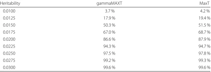
To evaluate the power, we create nine sets of data with GAMETES. Each set consists in 1000 datasets, all composed of 1000 individuals (500 cases and 500 controls) and 200 SNPs (out of which exactly one pair is linked with the trait). The heritability varies across the datasets from 0.03 to 0.01. In this way, we provide a range of decreasing effect sizes showing the power reduction. Table 10 indicates the percentage of time that the pair linked with the trait gave rise to an adjustedp-value below 5 %. We observe that the origi-nal MaxT and the new gammaMAXT algorithm leads to very similar power. By predicting theMi values instead of computing them explicitly, we can of course not win power, so that the power of the gammaMAXT algorithm is obviously equal or lower than the one of MaxT. However, we observe that the difference is small, the largest power reduction being of 1,7 %.
Conclusion
In this work we introduced gammaMAXT, a novel implementation of the maxT algorithm for multiple testing correction. The algorithm was implemented in software MBMDR-4.2.2, as part of the MB-MDR framework to screen for SNP-SNP, SNP-environment or SNP-SNP-environment interactions at a genome-wide level. In this context, we analyzed a dataset composed of 106SNPs and 1000 individuals within one day on a 256-core com-puter cluster. The same analysis would take about 104times longer with Van Lishout’s implementation of maxT, which was already an improvement of the classic Westfall and Young implementation [26]. These results are promising for future GWAIs. However,
Table 9Observed FWER ofMBMDR-4.2.2
Set Amount datasets Observed FWER
S1 1000 4.5 %
S2 1000 6.2 %
S3 200 7 %
Table 10Power comparison between the gammaMAXT and the MaxT algorithms
Heritability gammaMAXT MaxT
0.0100 3.7 % 4.2 %
0.0125 17.9 % 19.4 %
0.0150 50.3 % 51.5 %
0.0175 67.0 % 68.7 %
0.0200 86.6 % 87.9 %
0.0225 94.3 % 94.7 %
0.0250 97.5 % 97.8 %
0.0275 99.2 % 99.3 %
0.0300 99.6 % 99.6 %
the proposed gammaMAXT algorithm offers a general significance assessment and mul-tiple testing approach, applicable to any context that requires performing hundreds of thousands of tests. It offers new perspectives for fast and efficient permutation-based significance assessment in large-scale (integrated) omics studies.
Availability
MBMDR-4.2.2can be downloaded for free at http://www.statgen.ulg.ac.be.
Additional files
Additional file 1: Figure S1.Theoretical (green) versus predictedMivalues forD2. 10 % is again the optimal choice.
(EPS 64 kb)
Additional file 2: Figure S2.Theoretical (green) versus predictedMivalues forD3. 20 % is the optimal choice, but
10a low Kolmogorov-smirnov distance and remains a good choice. (EPS 64 kb)
Additional file 3: Figure S3.Theoretical (green) versus predictedMivalues forD4. 10 % is again the optimal choice.
(EPS 57 kb)
Competing interests
The authors declare that they have no competing interests.
Authors’ contributions
FVL and JHM discussed the pros and cons of Van Lishout’s implementation of MaxT. This lead to the idea to try to predict most of the computations. FVL first tried to base the predictions on a normal distribution without success. FG proved that a gamma distribution is a much better choice than a poisson, a normal, an exponential or a Weibull distribution. FVL and LW found the idea to focus on the top part of the distribution. KVS suggested to try to improve power by using either an extreme value distribution or a generalized gamma distribution. FVL found that a shifted gamma distribution is the best choice. KVS provided a lot of useful information for the background section. FVL carried out the analyses. KVS, FVL and LW interpreted the results. FVL and FG are the main contributors of the manuscript. All authors read and approved the final manuscript.
Acknowledgements
This research was in part funded by the Fonds de la Recherche Scientifique (F.N.R.S.), in particular “Integrated complex traits epistasis kit” (Convention 2.4609.11) [FVL, KVS]. We also acknowledge research opportunities offered by F.N.R.S., “Foresting in Integromics Inference” (Convention T.0180.13) [FG, KVS]. In addition, this paper presents research results of the Belgian Network DYSCO (Dynamical Systems, Control, and Optimization), funded by the Interuniversity Attraction Poles Programme, initiated by the Belgian State, Science Policy Office [FVL, FG, LW, KVS]. JHM was funded by National Institutes of Health (USA) grant LM009012. The scientific responsibility rests with the authors.
Author details
1Systems and Modeling Unit, Montefiore Institute, University of Liège, Allée de la découverte 10, 4000 Liège, Belgium. 2Bioinformatics and Modeling, GIGA-R, Avenue de l’Hôpital 1, 4000 Sart-Tilman, Belgium.3Institute for Biomedical
Informatics, Perelman School of Medicine, University of Pennsylvania, Philadelphia, PA 19104-6021, USA.
References
1. Shastry BS. Pharmacogenetics and the concept of individualized medicine. Pharmacogenomics J. 2006;6(1):16–21. 2. van’t Veer LJ, Bernards R. Enabling personalized cancer medicine through analysis of gene-expression patterns.
Nature. 2008;452(7187):564–70.
3. Galas DJ, Hood L. Systems biology and emerging technologies will catalyze the transition from reactive medicine to predictive, personalized, preventive and participatory (p4) medicine. Interdisc Bio Central. 2009;1:1–4.
4. Beevers CG, McGeary JE. Therapygenetics: moving towards personalized psychotherapy treatment. Trends Cogn Sci. 2012;16(1):11–12.
5. Lester KJ, Eley TC. Therapygenetics: Using genetic markers to predict response to psychological treatment for mood and anxiety disorders. Biology of mood and anxiety disorders. 2013;3(1):1–16.
6. Slatkin M. Epigenetic inheritance and the missing heritability problem. Genetics. 2009;182(3):845–50. 7. Eichler EE, Flint J, Gibson G, Kong A, Lean S, Moore JH, et al. Missing heritability and strategies for finding the
underlying causes of complex disease. Nat Rev Genet. 2010;11(6):446–50.
8. Lee SH, Wray NR, Goddard ME, Visscher PM. Estimating missing heritability for disease from genome-wide association studies. Am J Hum Genet. 2011;88(3):294.
9. Zuk O, Hechter E, Sunyaev SR, Lander ES. The mystery of missing heritability: Genetic interactions create phantom heritability. Proc Natl Acad Sci. 2012;109(4):1193–98.
10. Wan X, Yang C, Yang Q, Xue H, Fan X, Tang NL, et al. Boost: A fast approach to detecting gene-gene interactions in genome-wide case-control studies. Am J Hum Genet. 2010;87:325–40.
11. Gyenesei A, Moody J, Semple CA, Haley CS, Wei WH. High-throughput analysis of epistasis in genome-wide association studies with biforce. Bioinformatics. 2012;19:376–82.
12. Hemani G, Theocharidis A, Wei W, Haley C. epigpu: exhaustive pairwise epistasis scans parallelized on consumer level graphics cards. Bioinformatics. 2011;27:1462–1465.
13. Kam-Thong T, Czamara D, Tsuda K, Borgwardt K, Lewis C, Erhardt-Lehmann A, et al. epiblaster-fast exhaustive two-locus epistasis detection strategy using graphical pro- cessing units. Eur J Hum Genet. 2011;19:465–71. 14. Kam-Thong T, Azencott C, Cayton L, Putz B, Altmann A, Karbalai N, et al. Glide: Gpu-based linear regression for
detection of epistasis. Hum Hered. 2012;73:220–36.
15. Ritchie MD, Hahn LW, Moore JH. Power of multifactor dimensionality reduction for detecting gene-gene interactions in the presence of genotyping error, missing data, phenocopy, and genetic heterogeneity. Genet Epidemil. 2003;24(2):150–7.
16. Hahn LW, Ritchie MD, Moore JH. Multifactor dimensionality reduction software for detecting gene–gene and gene–environment interactions. Bioinformatics. 2002;19(3):376–82.
17. Calle ML, Urrea V, Vellalta G, Malats N, Van Steen K. Improving strategies for detecting genetic patterns of disease susceptibility in association studies. Stat Med. 2008;27:6532–546.
18. Cattaert T, Calle ML, Dudek SM, Mahachie John JM, Van Lishout F, Urrea V, et al. Model-based multifactor dimensionality reduction for detecting epistasis in case-control data in the presence of noise. Ann Hum Genet. 2011;75:78–89.
19. Gusareva E, Van Steen K. Practical aspects of genome-wide association interaction analysis. Hum Genet. 2014;133(11):1343-58.
20. Wienbrandt L, Kässens JC, Gonzalez-Dominguez J, Schmidt B, Ellinghaus D, Schimmler M. FPGA-based Acceleration of Detecting Statistical Epistasis in GWAS In: Science PC, editor. 14th International Conference on Computational Science. Elsevier - Procedia Computer Science, vol 29; 2014. p. 220–30. http://www.sciencedirect. com/science/article/pii/S1877050914001975.
21. Van Steen K. Traveling the world of gene-gene interactions. Brief Bioinform. 2011;13(1):1–19.
22. Mahachie John JM, Cattaert T, Van Lishout F, Gusareva E, Van Steen K. Lower-order effects adjustment in quantitative traits model-based multifactor dimensionality reduction. PLoS ONE. 2012;7(1):29594–1013710029594. 23. Van Lishout F, Mahachie John JM, Gusareva ES, Urrea V, Cleynen I, Théâtre E, et al. An efficient algorithm to
perform multiple testing in epistasis screening. BMC Bioinforma. 2013;14(138). http://www.biomedcentral.com/ 1471-2105/14/138.
24. Dunn OJ. Multiple comparisons among means. J Am Stat Assoc. 1961;56(293):52–64.
25. Ge Y, Dudoit S, Speed TP. Resampling-based multiple testing for microarray data analysis. Technical Report 633. Berkley: Department of Statistics, University of California; 2003.
26. Westfall PH, Young SS. Resampling-base Multiple Testing. New York: Wiley; 1993.
27. Mahachie John JM, Van Lishout F, Van Steen K. Model-based multifactor dimensionality reduction to detect epistasis for quantitative traits in the presence of error-free and noisy data. Eur J Hum Genet. 2011;19(6):696–703. 28. Calle ML, Urrea V, Malats N, Van Steen K. Mb-mdr: model-based multifactor dimensionality reduction for detecting
interactions in high-dimensional genomic data. Technical Report 24. 2008.
29. Mahachie John JM. Genomic association screening methodology for high-dimensional and complex data structures: Detecting n-order interactions. 2012. http://orbi.ulg.ac.be/handle/2268/136086.
30. Kotz S, Balakrishnan N, Johnson N. Continuous Multivariate Distributions, Models and Applications: Wiley; 2000. 31. Hautsch N, Malec P, Schienle M. Capturing the zero: A new class of zero- augmented distributions and
multiplicative error processes. J Financ Econ. 2013;12(1):89.
32. Bickel P, Doksum K. Mathematical Statistics, Basic Ideas and Selected Topics: Prentice-Hall, Inc; 1977.
33. Allenby GM, Leone RP, Jen LC. A dynamic model of purchase timing with application to direct marketing. J Am Stat Assoc. 1999;94:365–74.
34. Pattin KA, White BC, Barney N, Gui J, Nelson HH, Kelsey KT, et al. A computationally efficient hypothesis testing method for epistasis analysis using multifactor dimensionality reduction. Genet Epidemiol. 2009;33(1):87–94. 35. Minka TP. Estimating a gamma distribution. 2002. http://research.microsoft.com/en-us/um/people/minka/papers/
minka-gamma.pdf.
37. Libioulle C, Louis E, Hansoul S, Sandor C, Farnir F, Franchimont D, et al. Novel crohn disease locus identified by genome-wide association maps to a gene desert on 5p13.1 and modulates expression of ptger4. Plos Genetics. 2007;3(4):58.
38. Barett JC, Hansoul S, Nicolae DL, Cho JH, Duerr RH, Rioux JD, et al. Genome-wide association defines more than 30 distinct susceptibility loci for crohn’s disease. Nat Genet. 2008;40(8):955–62.
39. Urbanowicz RJ, Kiralis J, Sinnott-Armstrong NA, Heberling T, Fisher JM, Moore JH. Gametes: a fast, direct algorithm for generating pure, strict, epistatic models with random architectures. BioData Mining. 2012;5(1):16. http://www. ncbi.nlm.nih.gov/pubmed/23025260.
40. Bradley J. Robustness? Br J Math Stat Psychol. 1978;31:144–52.
Submit your next manuscript to BioMed Central and take full advantage of:
• Convenient online submission
• Thorough peer review
• No space constraints or color figure charges
• Immediate publication on acceptance
• Inclusion in PubMed, CAS, Scopus and Google Scholar
• Research which is freely available for redistribution