www.atmos-meas-tech.net/4/1161/2011/ doi:10.5194/amt-4-1161-2011
© Author(s) 2011. CC Attribution 3.0 License.
Measurement
Techniques
Analytical system for stable carbon isotope measurements of low
molecular weight (C
2
-C
6
) hydrocarbons
A. Zuiderweg, R. Holzinger, and T. R¨ockmann
Atmospheric Physics and Chemistry Group, Institute for Marine and Atmospheric research Utrecht, Utrecht University, Utrecht, The Netherlands
Received: 14 December 2010 – Published in Atmos. Meas. Tech. Discuss.: 11 January 2011 Revised: 2 June 2011 – Accepted: 8 June 2011 – Published: 22 June 2011
Abstract. We present setup, testing and initial results from a new automated system for stable carbon isotope ratio mea-surements on C2to C6atmospheric hydrocarbons. The inlet
system allows analysis of trace gases from air samples rang-ing from a few liters for urban samples and samples with high mixing ratios, to many tens of liters for samples from remote unpolluted regions with very low mixing ratios. The center-piece of the sample preparation is the separation trap, which is used to separate CO2and methane from the compounds of
interest. The main features of the system are (i) the capability to sample up to 300 l of air, (ii) long term (since May 2009) operationalδ13C accuracy levels in the range 0.3–0.8 ‰
(1-σ ), and (iii) detection limits of order 1.5–2.5 ngC (collected amount of substance) for all reported compounds.
The first application of this system was the analysis of 21 ambient air samples taken during 48 h in August 2009 in Utrecht, the Netherlands. Results obtained are generally in good agreement with those from similar urban ambient air studies. Short sample intervals allowed by the design of the instrument help to illustrate the complex diurnal be-havior of hydrocarbons in an urban environment, where di-verse sources, dynamical processes, and chemical reactions are present.
1 Introduction
A significant amount of the total reactive carbon input (esti-mated as near 1150 Tg yr−1, Guenther et al., 1995) to the at-mosphere consists of non-methane hydrocarbons (NMHCs).
Correspondence to: A. Zuiderweg
(azuider@gmail.com)
These are emitted to the atmosphere through many pro-cesses, both natural as a product of vegetative growth, de-cay and natural combustion of plant material, and anthro-pogenic including biomass burning for energy or heating, fossil fuel combustion, and industrial processes. Non-methane hydrocarbons play important roles in atmospheric chemistry contributing to the production of tropospheric ozone and resultant photochemical pollution, the forma-tion of aerosol particles, and the oxidative capacity of the atmosphere (Warneck, 1988; Seinfeld and Pandis, 1998; Goldstein and Galbally, 2007).
Low molecular weight NMHC, consisting of compounds with 2 to 7 carbon atoms (C2to C7), account for the vast
ma-jority of anthropogenic emissions to the troposphere (Mid-dleton, 1995). Acetylene, ethylene, propyne, and propylene originate primarily from combustion processes such as fos-sil fuel combustion and biomass burning; alkanes mainly stem from natural gas leakage and petroleum product evap-oration, with significant transportation sources as well; and aromatic compounds mainly from transportation sources and solvent evaporation (Goldstein and Shaw, 2003; Redeker et al., 2007). Oxidative processes provide the atmospheric moval mechanism of NMHC compounds, mainly through re-action with OH, which is by far the dominant process (Conny and Currie, 1996):
RH+OH→R+H2O (1)
Where R stands for any alkyl radical remaining after hydro-gen abstraction from the hydrocarbon RH. Other removal mechanisms include NO3, Cl, or O3 (Warneck, 1988;
Se-infeld and Pandis, 1998; Brenninkmeijer, 2009).
processes often act slightly differently on isotopologues and thus change the stable isotope ratio, which is expressed as
δ13C=
13C
[12C]
sample [13C]
[12C]
standard
−1
(2)
where measurements are referenced against a standard car-bon isotopic ratio, usually VPDB (Vienna Pee Dee Belem-nite). Measurements ofδ13C are commonly multiplied by 1000 ‰ for readability purposes (Goldstein and Shaw, 2003; Brenninkmeijer, 2009).
Isotopically lighter molecules usually react faster than iso-topically heavier ones. In the case of hydrocarbons, this is because bonds in molecules containing solely12C atoms are weaker than those containing one or more13C atoms. This causes small deviations from the original13C/12C ratio dur-ing chemical degradation. The ratio of the two rate coeffi-cients of the different isotopologues is known as a kinetic isotope effect (KIE).
KIE=k12
k13
. (3)
Knowledge of the KIE of relevant chemical reactions can provide a tool to improve the understanding of hydrocarbon atmospheric processing (Rudolph and Czuba, 2000).
Development of the coupled gas chromatography – (com-bustion interface) – isotope ratio mass spectrometer (IRMS), as pioneered by Matthews and Hayes (1978) for CO2 and
N2isotope work, substantially improved upon earlier
tech-niques based on dual-inlet isotope ratio mass spectrometers by greatly reducing necessary sample size and eliminating the need to extract individual compounds from a sample, which is a difficult and time-consuming task. This break-through allowed significant research work into the stable iso-topic ratios of carbon, nitrogen, oxygen and hydrogen con-taining compounds in the atmosphere.
Development of instrumentation able to accomplish com-pound specific measurement of carbon isotope ratios of NMHC is somewhat newer (Rudolph et al., 1997; Gold-stein and Shaw, 2003; Brenninkmeijer, 2009). Rudolph et al. (1997) developed the first instrument capable of com-pound specific stable carbon isotope ratio analysis measure-ments of multiple NMHCs. This instrument was initially used for observing carbon isotope ratios of emissions from biomass burning and transportation related sources, and ur-ban environment atmospheric samples. The observance of the magnitude of the kinetic isotope effect in hydrocarbon re-actions with OH and O3was also undertaken in subsequent
research with this instrument (Rudolph et al., 1997, 2002; Iannone et al., 2003; Anderson et al., 2004).
The availability of such measurements allowed the subse-quent development and application of the so-called isotopic
hydrocarbon clock approach, which is expressed as follows (Rudolph and Czuba, 2000):
δZ=tav·OHkZ·[OH]·OHKIEZ+0δZ (4)
whereδZ is the measured isotopic ratio of a compoundZ, tav the average age of the air mass,OHkZ the rate of
reac-tion of the compound with OH, [OH] the concentrareac-tion of OH,OHKIEZ the KIE in the reaction of compound Z with
OH, and0δZthe source isotope ratio of compoundZ; it may
also be further extended by adding terms representing reac-tions with e.g. O3 or Cl. This approach can improve
esti-mates of compound age compared to previous efforts, which relied on ratios of mixing ratios of two compounds emitted at the same time (Rudolph and Czuba, 2000). In the case of light non-methane hydrocarbons, the relatively short lifetime of these compounds in the atmosphere, from mere hours to tens of days, gives the possibility of utilizing the isotopic hy-drocarbon clock approach to constrain transport and aging in the atmosphere (Rudolph and Ehhalt, 1981; Rudolph et al., 2002; Goldstein and Shaw, 2003; Redeker et al., 2007).
Other applications of similar instruments that have been subsequently derived include measurements of NMHCδ13C in urban, marine and costal atmospheres and over the north Pacific and east Asia to evaluate atmospheric transport and airmass age (Tsunogai and Yoshida, 1999; Saito et al., 2002, 2009; Nara et al., 2007); of NMHC from biomass burning (Czapiewski et al., 2002; Nara et al., 2006); with some exten-sion, measurements of halocarbons and NMHC (Archbold et al., 2005; Redeker et al., 2007); specific measurement of chloromethane from plants and its atmospheric budget (Bill et al., 2002; Harper et al., 2003; Keppler et al., 2005); and measurement of leaf emissions of acetaldehyde to investi-gate biochemical reaction pathways (Jardine et al., 2009). Such measurements can be powerful tools to disentangle the relative contribution of different sources to the atmospheric burden of important atmospheric trace gases.
Here we present a new instrument that is capable of high-precision measurements of NMHC stable carbon isotope ra-tios. It has the unique capacity of being able to process very high volume samples of up to 300 l, such as those neces-sary for stable carbon isotope measurements of NMHC from very clean samples (e.g. stratospheric, firn air samples, or remote high volume air samples) and the flexibility of ac-cepting samples from many other sources. The system is constructed and tested to analyzeδ13C of non-methane hy-drocarbons from C2to C6, and methyl chloride.
2 Experimental
2.1 System description and procedure 2.1.1 The preconcentration system
of a variety of different samples. All cryotraps were oper-ated at 77 K and cooled with liquid nitrogen. If not speci-fied otherwise, electrical heating desorbed the trapped com-pounds. Helium was used as carrier gas to transfer the sample through the different components of the system. To allow the sampling of large volume samples, it is necessary to initially utilize large diameter cryotraps and progressively cryofocus to smaller volumes prior to GC injection. Cryogenic traps, when implemented properly, do not create isotopic fraction-ation (Archbold et al., 2005; Redeker et al., 2007). The fol-lowing parts of the preconcentration system are described be-low: (i) the primary cryogenic sampling trap (referred to as SAMP trap); (ii) the separation trap to separate CO2from the
NMHCs (referred to as SEP trap); (iii) the W-shaped cryo-genic recovery trap (REC trap); and (iv) the final cryocryo-genic focusing trap (FOC trap).
The SAMP trap is a 0.5 m×4 mm ID stainless-steel tube filled with 100/120 mesh glass-bead packing material, capa-ble of at least 100 standard ml min−1 (standard conditions are 0◦C, 1 bar) flow rates without loss. Typically this trap is operated at a flow of 50 standard ml min−1, which is main-tained by a MKS thermal mass flow-controller. A dual-head rotary pump (KNF Neuberger GmbH, Germany) draws the sample through the trap, and provides removal of bulk gases (mainly N2and O2). Desorption of any sample on the trap
is accomplished by heating it to 120◦C within 1 min after extraction.
The most innovative design feature of the preconcentration system is the method of CO2 removal. Whereas other
sys-tems (Rudolph et al., 1997; Tsunogai et al., 1999; Archbold et al., 2005) rely on chemical removal of any CO2employing
Carbosorb, Ascarite II or other sodium hydroxide-on-silica beads, here a packed stainless steel GC-column (Supelco Po-raPAK Q, 3 m×4 mm ID, 100/120 mesh) acted as a trap for NMHCs and allowed unwanted CO2to pass. We designed
the SEP trap as a non-chemical removal method to ensure ef-fective separation for large samples, i.e. samples with a high CO2 content. CO2 must be removed before IRMS
analy-sis can occur, because the target compounds are oxidized to CO2 for isotope analysis. In order to do so, the sample is
injected on this trap at 70 ml min−1with helium as the car-rier gas. The system procedure developed as a result of SEP trap testing (see Sect. 2.1.3, below) reverses the flow through the column after 10 minutes (any CO2having been vented)
to retrieve the compounds of interest from the column at a reduced helium flow rate (11.2 ml min−1). During recovery, the column is heated to and kept at 120◦C over a period of
40 min.
Before the sample material is recovered on the REC trap, any small remnant CO2and any H2O is removed in a small
glass reactor containing Ascarite II and Mg(ClO4)2. The
REC trap is a 0.7 m×2.5 mm ID W-shaped stainless steel cryotrap containing 100/120 mesh glass beads. After the re-covery time of 40 min, the REC trap is heated to 100◦C, thereby releasing the sample over the course of 5 min at
Table 1. Mean and standard deviation inδ13C ( ‰) SEP trap evaluation data.
No SEP No SEP Standard Standard
trapa trapa config.b config.b
Compound meanδ13C σ δ13C meanδ13C σ δ13C
Ethane −28.4 0.33 −28.6 0.27
Propane −34.6 0.49 −34.3 0.49
Methyl Chloride −46.4 0.69 −48.8 0.72
Benzene −27.4 0.36 −27.5 0.39
aSEP trap removed from system,n=10bStandard configuration, SEP trap installed,
n=10.
4.1 ml min−1 to the FOC trap, a 0.5 m×0.25 mm ID stain-less steel-jacketed capillary cryotrap. Sample injection into the GC occurs by extracting and heating the FOC trap to a temperature of over 100◦C within 30 s, at a flow rate of 2.1 ml min−1.
2.1.2 SEP trap verification and testing
Figure 2 displays a total ion abundance chromatogram demonstrating the separation properties of SEP trap under room temperature and aforementioned standard He flow rates of 70 ml min−1, utilizing a 200 ml 50:50 CO2/natural gas
testing mix and a quadrupole mass spectrometer as a detec-tor at the outlet of the SEP trap. Natural gas has a widely varying composition, but generally consists of methane (as bulk gas) and contains significant amounts of nitrogen, CO2,
and higher hydrocarbons such as ethane and propane ( ˇSkrbiæ and Zlatkoviæ, 1983; Milton et al., 2010). The injected mix-ture of natural gas and CO2as chosen here represents a test
of separation column performance of a very demanding sam-ple introduced on the system, representing the CO2content
of approximately 300 l of ambient air. Figure 2 shows that at 10 min after injection the bulk of methane, remnant nitro-gen (peak A) and CO2(peak B), has eluted while ethane and
other hydrocarbons (peak C) are still in the SEP trap. There-fore the system procedure has been set to reverse the flow through the column after 10 min to retrieve the compounds of interest, after venting all CO2.
Fig. 1. System diagram. A, B, C indicate Valco 6-port valves; SAMP, SEP, REC, and FOC indicate the primary sampling cryotrap, the
separation trap, the recovery cryotrap, and the focusing cryotrap, respectively. Mass flow controller (MFC) maximum flow rates are indicated in units of ml min−1(standard conditions).
1.E+04 1.E+05 1.E+06 1.E+07 1.E+08
0 2 4 6 8 10 12 14 16 18 20
Time after Injection (minutes)
A
bundance (counts)
A B C
Fig. 2. Performance of the separation trap. The identity of peaks A (methane and nitrogen), B (bulk carbon dioxide), and C (ethane and other
hydrocarbons) was confirmed by individual mass signals of the quadrupole mass spectrometer.
2.1.3 GC separation, combustion and detection
Gas chromatographic separation is done on a 52.5 m×0.25 mm Varian PoraPLOT Q GC column in a HP 5890 GC. The column is maintained at 40◦C for 10 minutes, thereafter being heated at a rate of 12◦C min−1 to
240◦C. This temperature is maintained for 35 min, giving a
The effluent from the GC column is roughly split 1:1 be-tween a quadrupole mass spectrometer (HP5970) for identi-fication of the compounds, and the remainder sent to a Ther-moFinnigan Delta+XP IRMS by way of a platinum-copper-nickel ceramic combustor (maintained at 900◦C and restored daily with O2), a nafion drier, and an open-split interface
(R¨ockmann et al., 2003). The actual flow into the IRMS is approximately 0.5 ml min−1. IRMSδ13C drift is monitored through direct injection of CO2via the open-split as a
work-ing standard. The stable carbon isotope ratio of this CO2has
been calibrated as−34.0 ‰±0.1 vs. VPDB by Rijksuniver-siteit Groningen, The Netherlands. Mixing ratios are cal-culated from the IRMS m/z 44 peak area measurements of each peak in the chromatogram, relative to peak areas from the working standard gas at accuracy levels of±10 % (see below). Mixing ratios of compounds not contained in the regularly measured working standard gas were estimated by extrapolation based on the number of carbon atoms in the molecules of the species in question and can therefore con-tain a larger systematic error (±30 %).δ13C values are calcu-lated from the individual ion signals of the IRMS, integrated per trace (m/z 44, 45, 46; automatic peak detection under nor-mal operation, manual evaluation if necessary), and mathe-matically corrected for17O through the ISODAT isotope ra-tio analysis package, utilizing the correcra-tion from Santrock et al. (1985).
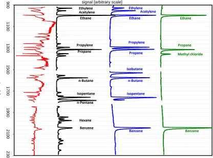
The sample chromatograms shown in Fig. 3 show the IRMS intensity traces at m/z 44 of two gas standards and an ambient air sample; and a 44/45 ratio trace for that ambient air sample, respectively, thus demonstrating the separation performance of the GC-IRMS system.
2.1.4 Ambient air sampling unit
As an addition to the basic system described above, a high-flow sampling unit (diagram Fig. 4) was developed allow-ing ambient air samplallow-ing at rates of up to 1 l min−1. The unit is set up as an auxiliary 2-stage cryogenic trapping system consisting of a large diameter stainless steel wa-ter trap (0.25 m×2.1 cm ID) and a stainless steel U-trap (0.5 m×1.0 cm ID) filled with glass beads (80/100 mesh). The water trap is constructed of 2.54 cm tubular stainless steel with large diameter Swagelok fittings and 0.32 cm (ID) stainless steel lines. The internal volume of this trap (approx-imately 100 ml) is large enough to freeze out water vapor from very large and humid air samples.
Sampling proceeds as follows: both traps are immersed in liquid nitrogen while flush gas (ultra pure synthetic air or nitrogen) is drawn through the system at 50 ml min−1by a dual head high-flow rotary pump downstream of the traps. The use of a pump keeps pressure inside the traps low at all times to prevent the condensation of oxygen. Once both traps are at temperature (approximately 2 min), the synthetic air supply is closed, the ambient sample line valve is opened, flow rates are increased to 0.5–1 l min−1 and sampling
be-gins. Following the sampling of the desired volume, the flow rate is reduced to 50 ml min−1, the sampling valve is closed, and the flush gas is reintroduced. Subsequently the pump valve is closed and the valve to the preconcentration system is opened and the traps are extracted from the liquid nitrogen in turn: first the water trap is removed and left to warm in lab-oratory ambient air for 5 min to reduce pressure effects from rapid warm up of such a large volume. Then it is inserted in a warm water bath at 40◦C to release adsorbed volatiles, while retaining water in liquid form at the bottom of the trap. The liberated volatiles are transferred to the large diameter U trap over 5 min. This trap is then extracted from the liq-uid nitrogen and allowed to warm in ambient laboratory air over 5 min, and is subsequently heated out under a 500◦C air stream for 5 min to transfer all sampled compounds to the preconcentration system.
2.1.5 Automatization
With the exception of the ambient air sampling unit, the sys-tem has fully automatic operation. Pneumatic lifters are used to move the traps in or out the Dewar vessels filled with liquid nitrogen. The traps, flow controllers, and valves are operated electronically via a process/time table. Autonomous opera-tion is limited to about 10 h by the supply of liquid nitrogen in the Dewar vessels.
2.2 Performance and stability
For calibration, a 9-compound reference gas (Apel-Riemer, AiR Environmental, Inc.) is used as the primary working standard. Of the compounds in this gas, 4 are monitored in test and calibration runs at the start and end of each mea-suring day, and during night (automated), namely ethane (206 ppb), propane (103 ppb), methyl chloride (103 ppb) and benzene (103 ppb). Calibration runs with the standard were done with varying volumes, either 50, 100, or 200 ml, to en-sure a range of peak areas similar to results in sample mea-surements and to test for non-linearity effects. Calibation runs using 100 ml of this gas were most commonly done. Usage of low volume high concentration calibration gas as compared to a high volume dilution of the same was found to have no effect in calibration results, similar to previous research (e.g. Archbold et al., 2005; Redeker et al., 2007), further verifying trap performance.
Theδ13C values of propane, methyl chloride, and benzene in the working standard were established utilizing the method described in Fisseha et al. (2009), at the Forschungszen-trum J¨ulich, Germany, to be−34.8±0.4, −48.7±0.4, and
−28.1±0.3 ‰ vs. VPDB, respectively. These calibration results agree (±0.3 to ±0.8 ‰, depending on compound) with all measurements of these compounds obtained by our system when calibrated against the aforementioned injected CO2, and taking into account the shift in methyl chloride.
9
0
0
1
1
0
0
1
3
0
0
1
5
0
0
1
7
0
0
1
9
0
0
2
1
0
0
2
3
0
0
tim
e
[s]
signal [arbitrary scale]
Fig. 3. Example chromatograms (IRMS, m/z 44 signal) of the working gas standard (green trace), the second calibration gas standard (blue
trace), and an ambient air sample (black trace), respectively. Peak identification of the ambient sample is based on retention time and the mass spectrum obtained with the quadrupole mass spectrometer. Additionally, the ambient air sample 44/45 ratio trace is provided (red trace) to demonstrate peak separation.
the other tested gases and the reference CO2give high
confi-dence that our estimate of−28.6±0.4 ‰ vs. VPDB is valid for ethane.
If the peak area of a given eluted compound was main-tained above 0.5 Vs, the IRMS measuredδ13C values showed no dependency on the sample size. Below this value peak in-tegration can yield inaccurate results and therefore a signal of 0.5 Vs was considered the limit of detection.
Figure 5 shows time series ofδ13C (‰) and system sensi-tivity to illustrate the long term stability of the system in the current configuration (since May 2009). The sensitivity was typically in the range 0.2–0.32 Vs ngC−1. Some variability is evident from Fig. 5b and can be attributed to the internal vari-ability of the filament emission in the IRMS. This variation is taken into account by referencing against the aforementioned gas standard. Repeatability of mixing ratio measurements is evaluated to be less than±5 % for all compounds. Together with the specified accuracy of±5 % for the gas standard this defines the overall error of±10 % for measured mixing ra-tios. The detection limit in terms of collected amount of carbon is calculated to be 1.5–2.5 ngC, based on the limit
of 0.5 Vs for the IRMS signal and the observed sensitivity range. Figure 5a illustrates also a drift ofδ13C in the system over the selected period. In order to correct for drift inδ13C, detrending is accomplished by observing weekly averages as compared to long-term calibration measurement means.
Fig. 4. Ambient air sampling unit. The water trap and the sample
trap are large diameter cryogenic stainless steel traps. Flush gas may be He, N2or synthetic air. Flows are regulated by a 5 l min−1
mass flow controller (MKS instruments). After extraction, the con-tents of the sample trap are flushed to the preconcentration system (Fig. 1).
The reproducibility for other compounds was tested by in-troducing another standard gas, containing 20 to 50 ppb of acetylene, ethylene, propylene and C4and C5saturated
hy-drocarbons (also see Fig. 3). The results of stability eval-uations of these compounds are broadly similar to those of the primary working standard. Table 2 summarizesδ13C and sensitivity means and 1-σ errors of all tested compounds.
3 First results
To demonstrate capabilities of this instrument, we present the results of a 48-h measurement campaign of selected non-methane hydrocarbons undertaken over 4–6 August 2009. Samples were taken from an ambient air inlet located∼20 m above ground level at 52◦0501400N, 5◦0905700E. The sam-pling location is within 500 m of a traffic highway, and is lo-cated outside our laboratory on the Utrecht University cam-pus, in a semi-urban environment. Thus, an abundance of
Table 2. Means and 1-σ standard deviations of δ13C ( ‰) and IRMS Sensitivity (Vs ngC−1)for compounds in regularly used cal-ibration gases.
δ13C mean Sensitivity mean Compound ±σ( ‰) ±σ (Vs ngC−1)
Primary NMHC working standarda
Ethane −28.898±0.284 0.249±0.0053 Propane −34.716±0.397 0.254±0.0063 MeCl −48.528±0.795 0.231±0.0058 Benzene −27.915±0.484 0.302±0.0083
Other tested compoundsb
Acetylene −40.922±0.441 0.241±0.0062 Ethylene −36.307±0.716 0.239±0.010 Propylene −32.955±0.658 0.258±0.010 Isobutane −32.209±0.542 0.271±0.0097 Butane −35.658±0.476 0.273±0.0083 Isopentane −34.927±0.308 0.33±0.0095
a9-month detrended long-term accuracy levelsbn=20, over period of 1 month.
local sources, dominated by traffic emissions, can be ex-pected for hydrocarbons. Atmospheric conditions at the time of the campaign were characterized by warm stable sum-mer weather. During this period, high surface pressure was located above the North Sea. The sample days were simi-lar meteorologically, with clear skies, light winds, and high temperatures near 30◦C. At night, temperatures decreased to near 20◦C and the winds became near calm.
The samples were taken and processed in situ using the aforementioned ambient sampling unit, with 20 l samples (sampling rate 0.5 l min−1)taken at approximately 2-h inter-vals (excepting necessary calibration runs of the instrument) and processed immediately. The short time interval between samples afforded by the instrument design allowed detailed insight into diurnal evolution of NMHCδ13C; more so than the majority of previous urban stable carbon isotope studies. The 20 l sample size was chosen to ensure IRMS peak areas of>0.5 Vs for the all hydrocarbons of interest.
3.1 Mixing ratio
Day since Jan 1 2009
d
e
lt
a
1
3
C
(
p
e
rm
il)
d
if
fe
re
n
c
e
f
ro
m
m
e
a
n
200 250 300 350 400
-4
-2
0
2
4
Ethane Propane Methyl Chloride Benzene 50mL
100mL 200mL
A
Day since Jan 1 2009
P
e
a
k
a
re
a
p
e
r
n
g
C
a
rb
o
n
(
V
s
/n
g
C
)
200 250 300 350 400
0
.1
0
0
.2
0
0
.3
0
0
.4
0
B
Fig. 5. Time-stability of the system. Panels A and B show the difference from mean ofδ13C ( ‰, panel A); and sensitivity (Vs ngC−1, panel
B) of the 4 tested compounds in the working gas standard, respectively. Data of various injection volumes (50, 100, and 200 ml) are plotted.
The lines in panel A represent linear fits; the horizontal lines in panel B do not represent any trend but are plotted to make the long term variability more visible.
of the boundary layer mixing height. Morning vehicular traf-fic is intense; heavy congestion on local highways is com-mon in the periods from 07:00 to 09:00 (all times in Central European Summer Time). The afternoon-evening (16:00 to 18:00) peak of traffic, though generally less intense than that of the morning but still notable, is not clearly observed in the data. This is attributed to increased mixing in the after-noon due to the breakup of the nighttime boundary layer, as compared to the morning hours.
Ethane also displays a clear diurnal cycle, but in con-trast to the above compounds has peaks in mixing ratio dur-ing the night and early morndur-ing, far earlier than other com-pounds. The prevailing meteorological conditions of (near) calm winds during night suppressed mixing and allowed the buildup of continuously emitted gasses. Presuming that the main urban source of ethane is leakage of natural gas, local leakage could cause such an increase of mixing ratio. The daytime decrease may be similarly ascribed to the increase in mixing and dilution.
Isopentane, hexane, and benzene show profiles similar to the unsaturated hydrocarbons mentioned above. The change in mixing during daytime and nighttime can help to explain the afternoon decrease and nighttime buildup in mixing
ra-tio of all alkanes measured, with the excepra-tion of n-pentane (Fig. 7h), which exhibits larger daytime than night-time mix-ing ratios. This implies a different, non-local source that dominates the mixing ratios for this compound. Supporting evidence for a distinct and non-local source can be found in the stable isotope measurements of this compound, of which discussion follows.
3.2 Stable carbon isotope composition
Figure 8a–j showsδ13C measurements over the sampling pe-riod. In general,δ13C averages over the 48-h period (Table 4) agree well with published values from studies of urban air.
Acetylene has a large daily variation (maximum of 5 ‰ and minimum of−15 ‰), but its mean over the entire period is−9.1 ‰, which falls well in the urban range of−8±4 ‰ as reported in Goldstein and Shaw (2003). The maximum observed in acetylene is more enriched than previous mea-surements reported in urban environments, but is within the range of daytime summer values reported from rural/marine environments (Redeker et al., 2007).
d13C (permil)
C
o
u
n
t
-30.0 -29.5 -29.0 -28.5 -28.0
0
5
1
0
1
5
2
0
2
5
3
0
A) Ethane
stdev = 0.284
mean = -28.898 All Volumes
50mL 100mL 200mL
d13C (permil)
C
o
u
n
t
-36 -35 -34 -33
0
5
1
0
1
5
2
0
2
5
3
0
B) Propane
stdev = 0.397 mean = -34.716
d13C (permil)
C
o
u
n
t
-51 -50 -49 -48 -47 -46
0
5
1
0
1
5
C) Methyl Chloride
stdev = 0.795 mean = -48.528
d13C (permil)
C
o
u
n
t
-30 -29 -28 -27 -26
0
5
1
0
1
5
2
0
D) Benzene
stdev = 0.484 mean = -27.915
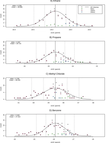
Fig. 6. Histograms of detrendedδ13C ( ‰) data, together with Gaussian fit for the Apel-Riemer (AiR) multicompound NMHC calibration gas, including measurements of various volumes (50, 100, 200 ml) for peak area ranges comparable to measurements. Dashed lines indicate 1 and 2σ intervals.
−17 ‰), agrees with expected mean values for C2 to C5
alkenes (−22±8 ‰, Goldstein and Shaw, 2003). The large diurnal variation, can be expected for such a reac-tive compound with a high KIE (18.6 ‰, Anderson et al., 2004). Strong fractionation occurs during summer day-light hours when OH levels are considerably high. Uti-lizing the isotopic clock parameterization (Eq. 4, Rudolph
and Czuba, 2000) provides additional support for this: as-suming that the nighttime δ13C value (mean −27 ‰) and daytime value (mean −10 ‰) represent the unoxi-dized (0δC2H4)and oxidized (δC2H4)isotope ratios of
ethy-lene, respectively, a value for OHKIEC2H4 of 18.6 ‰ and OHk
C2H4= 7.9×10⁻¹²cm3s−1 (at 296 K, Atkinson et al.,
5 10 15 20 0 .0 0 .4 0 .8 1 .2 V M R ( p p b )
A) Acetylene All
Day 1 Day 2
5 10 15 20
0 .0 1 .0 2 .0 B) Ethylene
5 10 15 20
0 2 4 6 8 V M R ( p p b ) C) Ethane
5 10 15 20
0 .0 0 .2 0 .4 0 .6 D) Propylene
5 10 15 20
0 2 4 6 8 1 0 1 2 V M R ( p p b ) E) Propane
5 10 15 20
0
1
2
3 F) n-Butane
5 10 15 20
0 .0 0 .5 1 .0 1 .5 2 .0 V M R ( p p b ) G) Isopentane
5 10 15 20
0 .0 0 .4 0 .8 H) n-Pentane
5 10 15 20
0 .0 0 .1 0 .2 0 .3 0 .4
Local Time (Hours)
V M R ( p p b ) I) Hexane
5 10 15 20
0 .0 0 .2 0 .4 0 .6
Local Time (Hours) J) Benzene
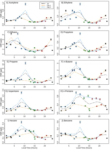
Fig. 7. Mixing ratios (ppb) versus time over 48-h (4–6 August 2009) period, overlapped on one diurnal cycle. Error bars indicate the 10 %
accuracy levels. Period means in Table 3. Colors indicate time periods: P1 (black): 21:00–05:00; P2 (blue): 05:00–11:00; P3 (green): 11:00– 15: 30; P4 (red): 15:30–21:00; these correspond to time period colors in Figs. 8 and 9. Period codes correspond to those in Tables 3, 4, and 5. Dashed lines are running averages.
fractionation is 3.6×10⁶molecules cm−3 for a 9 h atmo-spheric processing time. This OH concentration is well within the range for summer tropospheric conditions (e.g., Lu and Khalil, 1991).
The ethane stable isotope ratios we measured are in gen-eral more enriched than higher alkanes. This is due to its dif-fering source from natural gas, the ethane in which is known to be relatively enriched. The meanδ13C of ethane was
Table 3. Mean mixing ratio and sample standard deviation, 48-h measurements, 4 to 6 August 2009.
Mean VMR σ Mean VMR σ Mean VMR σ Mean VMR σ Mean VMR σ
Compound all (ppbv) (ppbv) P1a(ppbv) (ppbv) P2 (ppbv) (ppbv) P3 (ppbv) (ppbv) P4 (ppbv) (ppbv)
Acetylene 0.29 0.22 0.26 0.07 0.51 0.36 0.15 0.01 0.22 0.09
Ethylene 0.77 0.62 0.88 0.48 1.45 0.71 0.33 0.10 0.40 0.27
Ethane 3.09 2.23 4.52 2.43 3.98 2.68 1.41 0.69 2.14 1.03
Propylene 0.21 0.14 0.21 0.08 0.36 0.19 0.11 0.02 0.16 0.05
Propane 2.02 2.14 1.83 0.77 3.87 3.88 1.41 0.90 0.99 0.45
n-Butane 1.19 0.67 1.13 0.47 2.03 0.74 0.77 0.17 0.85 0.38
Isopentane 0.42 0.34 0.31 0.12 0.76 0.58 0.31 0.08 0.30 0.09
n-Pentane 0.45 0.27 0.23 0.10 0.61 0.31 0.43 0.30 0.55 0.17
Hexane 0.16 0.09 0.12 0.03 0.25 0.11 0.18 0.08 0.11 0.03
Benzene 0.20 0.11 0.24 0.07 0.27 0.21 0.12 0.03 0.17 0.06
aPeriod codes are the same as those defined in Fig. 7.
Table 4. Meanδ13C ( ‰) vs. VPDB and sample standard deviation, 48-h measurements, 4 to 6 August 2009.
Meanδ13C σ Meanδ13C σ Meanδ13C σ Meanδ13C σ Meanδ13C σ
Compound (‰) all (‰) P1a(‰) (‰) P2 (‰) (‰) P3 (‰) (‰) P4 (‰) (‰)
Acetylene −9.1 4.4 −10.2 1.4 −10.2 4.8 −6.2 6.8 −9.6 2.8 Ethylene −17.0 7.9 −23.3 3.2 −21.5 5.3 −9.1 4.2 −11.7 6.1 Ethane −24.5 0.6 −24.1 0.5 −24.6 0.8 −24.6 0.8 −24.6 0.17 Propylene −21.1 2.3 −21.7 1.3 −19.6 2.5 −20.3 2.5 −22.8 2.1 Propane −27.9 1.7 −27.0 2.3 −27.8 1.4 −28.6 1.7 −28.3 1.1 n-Butane −27.6 1.7 −27.0 1.4 −26.2 1.3 −29.3 1.3 −27.8 1.1 Isopentane −29.0 0.6 −29.0 0.8 −29.0 0.6 −29.4 0.6 −28.9 0.3 n-Pentane −27.0 1.6 −28.0 1.2 −28.2 0.9 −26.0 2.0 −25.8 0.4 Hexane −30.4 3.7 −28.6 1.7 −32.1 7.4 −29.4 1.0 −30.7 1.0 Benzene −26.2 2.3 −25.9 1.4 −26.8 5.1 −25.5 1.6 −26.7 0.2
aPeriods are the same as in Table 3.
Theδ13C of the C3to C6alkanes (with the exception of
n-butane and n-pentane, see below) show little (clearly appar-ent) diurnal variation and mean values of−27 to−30 ‰ dur-ing all periods. Previously reported measurements indicated
−27±2.5 ‰ (Rudolph et al., 2002; Goldstein and Shaw, 2003). The presence of a single very depleted point (−45 ‰) in measurements of hexane is notable, but this outlier may be due to an unidentified experimental problem. Apart from this point, standard deviations for these compounds also cor-respond well to previous results. Benzene also fits well to previous measurements despite some apparent high morning variability: mean−26.2±2.3 ‰, compared to literature val-ues of−27±2 ‰ (Goldstein and Shaw, 2003).
3.3 Source signatures
A common tool for atmospheric isotope research to deci-pher sources is the Keeling plot analysis, which was first developed for the analysis of stable carbon isotopes of car-bon dioxide (Keeling, 1958). This involves correlatingδ13C against the inverse of the mixing ratio, and linearly
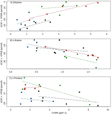
fit-ting the result. The y-intercept of this fit then indicates the isotopic composition of the contaminating source that mixes into background air. This procedure is based on a few assumptions, most importantly: (1) there should be only one source and a stable reservoir into which it is being di-luted; and (2) the δ13C and inverse mixing ratio should be well-correlated; lest the values calculated become unclear and unreliable (Keeling, 1958). In our dataset, the Keel-ing plot analysis works well for ethylene, butane, and n-pentane (Fig. 9a–c). The isotope source signatures deter-mined this way are given in Table 5. Other measured com-pounds are not included because of small isotopic variation or low correlation, indicating that the above conditions are violated.
5 10 15 20
-30
-20
-10
0
10
d13C v. VPDB (permil)
A) Acetylene All
Day 1 Day 2
5 10 15 20
-30
-20
-10
0 B) Ethylene
5 10 15 20
-28
-26
-24
-22
-20
d13C v. VPDB (permil)
C) Ethane
5 10 15 20
-26
-24
-22
-20
-18
-16 D) Propylene
5 10 15 20
-32
-30
-28
-26
-24
d13C v. VPDB (permil)
E) Propane
5 10 15 20
-32
-30
-28
-26
-24
F) n-Butane
5 10 15 20
-34
-32
-30
-28
-26
-24
d13C v. VPDB (permil)
G) Isopentane
5 10 15 20
-32
-30
-28
-26
-24
-22 H) n-Pentane
5 10 15 20
-50
-40
-30
-20
-10
Local Time (Hours)
d13C v. VPDB (permil)
I) Hexane
5 10 15 20
-35
-30
-25
-20
Local Time (Hours)
J) Benzene
Fig. 8. Compoundδ13C ( ‰ vs. VPDB) vs. time (hours) over 48-h (4–6 August 2009) period, overlapped. Error bars indicate 1-σ ranges. Period means and standard deviations in Table 4. Colors of points denote the time periods, which are defined in Fig. 7.
The interpretation for n-butane and n-pentane is more complicated because their lifetimes are longer. As a re-sult their mixing ratios are controlled by transport and mixing of different sources. The source signatures of n-butane during periods 3 and 4 (−25.4 and −24.5 ‰, re-spectively) suggest that emissions from fossil fuel combus-tion (-27±2.5 ‰, Goldstein and Shaw, 2003) are the domi-nant local source. However, the reversed slope may indicate that background concentrations of n-butane originate mainly from other sources.
0 1 2 3 4 5 6
-2
5
-2
0
-1
5
-1
0
-5
d
1
3
C
v
.
V
P
D
B
(
p
e
rm
il)
A) Ethylene
0.0 0.5 1.0 1.5
-3
0
-2
8
-2
6
d
1
3
C
v
.
V
P
D
B
(
p
e
rm
il)
B) n-Butane
0 2 4 6 8 10
-2
9
-2
7
-2
5
1/VMR (ppb^-1)
d
1
3
C
v
.
V
P
D
B
(
p
e
rm
il)
C) n-Pentane
Fig. 9. Ethylene, n-butane, and n-pentaneδ13C ( ‰ vs. VPDB) plotted versus inverse mixing ratio (ppb−1)over the 48-h (4–6 August 2009) period, with linear fits to points of each time period. Derived values for isotope source signatures are given in Table 5. Colors indicate periods as indicated in Fig. 7.
Table 5. Source signature (SS, in ‰ vs. VPDB) andr2from fits in Fig. 9, 48-h measurements, 4 to 6 August 2009.
Compound SS all ( ‰) R2all SS P1a( ‰) R2P1 SS P2 ( ‰) R2P2 SS P3 ( ‰) R2P3 SS P4 ( ‰) R2P4 Ethylene −26.8 0.68 −29.8 0.76 −25.7 0.17 −12.6 0.04 −22.7 0.89 n-Butane −24.7 0.52 −26 0.07 −24.7 0.29 −25.4 0.47 −24.5 0.98 n-Pentane −25.9 0.22 −27 0.17 −27.8 0.08 −23.9 0.65 −26 0.03
aPeriods are the same as in Table 3.
4 Conclusions
We have presented a NMHC stable carbon isotope analy-sis system capable of high-resolution measurements of many compounds from a large variety of sample sources with small measurement errors (1 ‰ vs. VPDB or less). In particular, the capability to process high volume atmospheric allows ex-amination of samples with large quantities of bulk gases and
CO2, without loss of any compounds of interest, and with
Acknowledgements. We would like to thank Henk Jansen, of
Rijksuniversiteit Groningen, The Netherlands, for calibration of the CO2reference standard; and Iulia Gensch, of Forschungscentrum J¨ulich, Germany, for calibration of the NMHC working standard.
Edited by: D. Riemer
References
Anderson, R. S., Huang, L., Iannone, R., Thompson, A. E., and Rudolph, J.: Carbon kinetic isotope effects in the gas phase reac-tions of light alkanes and ethene with the OH radical at 296±4 K, J. Phys. Chem. A, 108, 11537–11544, doi:10.1021/JP0472008, 2004.
Archbold, M. E., Redeker, K. R., Davis, S., Elliot, T., and Kalin, R. M.: A method for carbon stable isotope analysis of methyl halides and chlorofluorocarbons at pptv concentrations, Rapid Commun. Mass Sp., 19, 337–340, doi:10.1002/rcm.17, 2005. Atkinson, R., Baulch, D. L., Cox, R. A., Crowley, J. N.,
Hamp-son, R. F., Hynes, R. G., Jenkin, M. E., Rossi, M. J., Troe, J., and IUPAC Subcommittee: Evaluated kinetic and photochemi-cal data for atmospheric chemistry: Volume II - gas phase re-actions of organic species, Atmos. Chem. Phys., 6, 3625–4055, doi:10.5194/acp-6-3625-2006, 2006.
Bill, M., Rhew, R. C., Weiss, R. F., and Goldstein, A. H.: Car-bon isotope ratios of methyl bromide and methyl chloride emit-ted from a coastal salt marsh, Geophys. Res. Lett., 29(4), 4 pp., doi:10.1029/2001GL012946, 2002.
Brenninkmeijer, C. A. M.: Applications of stable isotope analysis to atmospheric trace gas budgets, Eur. Phys. J. C, 1, 137–148, doi:10.1140/epjconf/e2009-00915-x, 2009.
Conny, J. M. and Currie, L. A.: The isotopic characterization of methane, non-methane hydrocarbons and formadehyde in the troposphere, J. Atmos. Environ., 30(4), 621–638, 1996. Czapiewski, K. V., Czuba, E., Huang, L., Ernst, D., Norman, A. L.,
Koppmann, R., and Rudolph, J.: Isotopic composition of non-methane hydrocarbons in emissions from biomass burning, J. At-mos. Chem., 43, 45–60, 2002.
Fisseha, R., Spahn, H., Wegener, R., Hohaus, T., Brasse, G., Wis-sel, H., Tillmann, R., Wahner, A., Koppmann, R., and Kiendler-Scharr, A.: Stable carbon isotope composition of secondary or-ganic aerosol fromβ-pinene oxidation, J. Geophys. Res., 114, D02304, doi:10.1029/2008JD011326, 2009.
Goldstein, A. H. and Galbally, I. E.: Known and unexplored organic constituents in the Earth’s atmosphere, Environ. Sci. Technol., 41(5), 1514–1521, doi:10.1021/es072476p, 2007.
Goldstein, A. H. and Shaw, S. L.: Isotopes of volatile organic com-pounds: an emerging approach for studying atmospheric budgets and chemistry, Chem. Rev., 103, 5025–5048, 2003.
Guenther, A., Hewitt, C. N., Erickson, D., Fall, R., Geron, C., Graedel, T., Harley, P., Klinger, L., Lerdau, M., McKay, W. A., Pierce, T., Scholes, B., Steinbrecher, R., Tallamraju, R., Tay-lor, J., and Zimmerman, P.: A global-model of natural volatile organic-compound emissions, J. Geophys. Res.-Atmos., 100, 8873–8892, 1995.
Harper, D. B., Hamilton, J. T. G., Ducrocq, V., Kennedy, J. T., Downey, A., and Kalin, R. M.: The distinctive isotopic signa-ture of plant-derived chloromethane: possible application in
con-straining the atmospheric chloromethane budget, Chemosphere, 52, 433–436, doi:10.1016/S0045-6535(03)00206-6, 2003. Iannone, R., Anderson, R. S., Rudolph, J., Huang, L., and Ernst, D.:
The carbon kinetic isotope effects of ozone-alkene reactions in the gasphase and the impact of ozone reactions on the stable car-bon isotope ratios of alkenes in the atmosphere. Geophys. Res. Lett., 30(13), 1684–1688, doi:10.1029/2003GL017221, 2003. Jardine, K. J., Karl, T., Lerdau, M., Harley, P., Guenther, A., Mak, J.
E.: Carbon isotope analysis of acetaldehyde emitted from leaves following mechanical stress and anoxia, Plant Biology, 11(4), 591–597, doi:10.1111/j.1438-8677.2008.00155.x, 2009. Keeling, C. D.: The concentration and isotopic abundances of
at-mospheric carbon dioxide in rural areas, Geochim. Cosmochim. Acta, 13, 322–334, 1958.
Keppler, F., Harper, D. B., R¨ockmann, T., Moore, R. M., and Hamil-ton, J. T. G.: New insight into the atmospheric chloromethane budget gained using stable carbon isotope ratios, Atmos. Chem. Phys., 5, 2403–2411, doi:10.5194/acp-5-2403-2005, 2005. Lu, Y. and Khalil, M. A. K.: Tropospheric OH: model calculations
of spatial, temporal, and secular variations, Chemosphere, 23, 397–444, 1991.
Matthews, D. M. and Hayes, J. M.: Isotope-ratio-monitoring gas chromatography-mass spectrometry, Anal. Chem., 50(11), 1465–1473, 1978.
Middleton, P.: Sources of air pollutants, in: In Composition, Chem-istry, and Climate of the Atmosphere, edited by: Singh, H. B., John Wiley & Sons Inc., New York, 88–119, 1995.
Milton, M. J. T., Harris, P. M., Brown, A. S., and Cowper, C. J.: Normalization of natural gas composition data mea-sured by gas chromatography, Meas. Sci. Technol., 20, 025101, doi:10.1088/0957-0233/20/2/025101, 2010.
Nara, H., Nakagawa, F., and Yoshida, N.: Development of two-dimensional gas chromatography/ isotope ratio mass spectrome-try for the stable carbon isotopic analysis of C2–C5 non methane hydrocarbons emitted from biomass burning, Rapid Commun. Mass Sp., 20, 241–247, doi:10.1002/rcm.2302, 2006.
Nara, H., Toyoda, S., and Yoshida, N.: Measurements of stable car-bon isotopic composition of ethane and propane over the West-ern North Pacific and EastWest-ern Indian Ocean: a useful indicator of atmospheric transport process, J. Atmos. Chem., 56, 293–314, doi:10.1007/s10874-006-9057-3, 2007.
Redeker, K. R., Davis, S., and Kalin, R. M.: Isotope values of atmospheric halocarbons and hydrocarbons from Irish urban, rural, and marine locations, J. Geophys. Res., 112, D16307, doi:10.1029/2006JD007784, 2007.
R¨ockmann, T., Kaiser, J., Brenninkmeijer, C. A. M., and Brand, W. A.: Gas-chromatography, isotope-ratio mass spectrometry method for high-precision position-dependent15N and18O mea-surements of atmospheric nitrous oxide, Rapid Commun. Mass Spectrom., 17, 1897–1908, 2003.
Rudolph, J. and Czuba, E.: On the use of isotopic composition measurements of volatile organic compounds to determine the “photochemical age” of an air mass, Geophys. Res. Lett., 27(23), 3865–3868, 2000.
Rudolph, J. and Ehhalt, D. H.: Measurements of C2–C5 hydrocar-bons over the North Atlantic, J. Geophys. Res., 86(C12), 11959– 11964, 1981.
organic compunds at ppt levels in ambient air, Geophys. Res. Lett., 24(6), 659–662, 1997.
Rudolph, J., Czuba, E., Norman, A. L., Huang, L., and Ernst, D.: Stable carbon isotope composition of nonmethane hydrocar-bons in emissions from transportation related sources and atmo-spheric observations in an urban atmosphere, Atmos. Environ., 36, 1173–1181, 2002.
Saito, T., Tsunogai, U., Kawamura, K., Nakatsuka, T., and Yoshida, N.: Stable carbon isotopic compositions of light hy-drocarbons over the Western North Pacific and implication for their photochemical ages, J. Geophys. Res., 107(D4), 4040, doi:10.1029/2000JD000127, 2002.
Saito, T., Kawamura, K., Tsunogai, U., Chen, T., Matsueda, H., Nakatsuka, T., Gamo, T., Uematsu, M., and Huebert, B. J.: Pho-tochemical histories of nonmethane hydrocarbons inferred from their stable carbon isotope ratio measurements over east Asia, J. Geophys. Res., 114, D11303, doi:10.1029/2008JD011388, 2009.
Santrock, J., Studley, S. A., and Hayes, J. M.: Isotopic analyses based on the mass spectra of carbon dioxide, Anal. Chem., 57(7), 1444–1448, doi:10.1021/ac00284a060, 1985.
Seinfeld, J. H. and Pandis, S. N.: Atmospheric Chemistry and Physics: from Air Pollution to Climate Change, John Wiley and Sons, New York, 1326 pp., 1998.
Skrbic, B. D. and Zlatkovic, M. J.: Simple method for the rapid analysis of natural gas by gas chromatography, Chro-matographia, 17(1), 44–46, 1983.
Tsunogai, U. and Yoshida, N.: Carbon isotopic compositions of C2–C5 hydrocarbons and methyl chloride in urban, coastal, and maritime atmospheres over theWestern North Pacific, J. Geo-phys. Res., 104(D13), 16033–16039, 1999.