R E S E A R C H
Open Access
Self-organization of developing embryo using
scale-invariant approach
Ali Tiraihi
1, Mujtaba Tiraihi
2and Taki Tiraihi
3** Correspondence: ttiraihi@gmail. com
3Department of Anatomical
Sciences, Faculty of Medical Sciences, Tarbiat Modares University, Tehran, Iran Full list of author information is available at the end of the article
Abstract
Background:Self-organization is a fundamental feature of living organisms at all hierarchical levels from molecule to organ. It has also been documented in developing embryos.
Methods:In this study, a scale-invariant power law (SIPL) method has been used to study self-organization in developing embryos. The SIPL coefficient was calculated using a centro-axial skew symmetrical matrix (CSSM) generated by entering the components of the Cartesian coordinates; for each component, one CSSM was generated. A basic square matrix (BSM) was constructed and the determinant was calculated in order to estimate the SIPL coefficient. This was applied to developing C. elegansduring early stages of embryogenesis. The power law property of the method was evaluated using the straight line and Koch curve and the results were consistent with fractal dimensions (fd). Diffusion-limited aggregation (DLA) was used to validate the SIPL method.
Results and conclusion:The fractal dimensions of both the straight line and Koch curve showed consistency with the SIPL coefficients, which indicated the power law behavior of the SIPL method. The results showed that the ABp sublineage had a higher SIPL coefficient than EMS, indicating that ABp is more organized than EMS. The fd determined using DLA was higher in ABp than in EMS and its value was consistent with type 1 cluster formation, while that in EMS was consistent with type 2.
Background
Self-organization is a property of the biological structure [1] and is reported to be important in protein folding [2-4]. It has also been documented that at higher hier-archical levels such as the organelle level, it has a crucial role in the biogenesis of secretory granules in the Golgi apparatus [5,6]. Martin and Russell have shown that self-organization exists in mitochondria, where redox reactions are localized [7]. The most obvious example of self-organization at the organelle level is the cytoskeleton during the mitotic cycle, where mitotic spindle forms dynamically [8] using molecular motors [9]. Misteli concluded that self-organization could govern the mechanistic prin-ciples of cellular architecture [10]. The multicellular embryo develops from a zygote, characterized by a dynamic self-organizing process [11].
At an early stage of embryonic development, the forming cells adhere to each other [12] with coordinated cellular movement to form the primary embryonic body axis [13]. These movements are self-regulated and lead to a defined pattern [14]. In vitro
studies have confirmed self-organization in human embryonic stem cell (hESC) differen-tiation, resulting in the formation of the three germ layers and gastrulation [15]. Ungrin et al. reported a similar finding in the morphogenesis of hESCs cultured in suspension, which yielded embryoid bodies [16] with the property of self-organization. At later developmental stages such as organogenesis, Schiffmann reported self-organization in driving gastrulation and organ formation [17], where the increase in the mass of the organ and its cell number reportedly contribute to organogenesis [18]. Moreover, in vitro organogenesis showed a mechanism similar to that in vivo [19]. Among the factors contributing to organogenesis is self-organization; for example, in vitro organogenesis of the cultured mouse submandibular salivary gland at embryonic day 13 retains the capacity for branching, and when it is co-cultured with mesenchymal tissues, morpholo-gical differentiation of the gland results [20]. Similar results were obtained with cultured embryonic kidney explants leading to nephronal differentiation [21]. Other investigators introduced developmental self-organization in order to evaluate the morphogenesis of the embryo [22]. While the development of the embryo from a zygote to a multicellular organism is characterized by a dynamic self-organizing process [11], the emergence of an organized system is also associated with the expression of gene networks [23]. This could demonstrate the advantage of applying self-organization to cellular events [24]. In the present study, early development ofC. elegans was investigated as an example of self-organization using a scale-invariant power law to evaluate the self-organizing properties of two sublineages with different differentiation fates.
Two features should be considered in the quantitative validation of a self-organization process in a developing embryo. First, the different scales of the animal body; for exam-ple, Waliszewski et al. reported that the microscopic gene expression and the macro-scopic cellular proliferation were scale-invariant systems [25], the scale-free feature of which was shown to result in the emergence of organizational dynamics at all hierarchi-cal levels of the living matter [26]. Secondly, metazoan cells develop from a single cell, and this involves complex spatio-temporal events [11,27].
Moreover, Molski and Konarski revealed that the fractal structure of the space in any biological system could characterize self-organization [28]. The fractal method can be used to describe the irregularity of shapes that cannot be formulated in Euclidean geo-metry. It is characterized by self-similarity [29], and describes spatial structure in a scale free measure [30]. In this study, the development ofC. elegansembryos was evaluated at different time frames (stages) using a scale free power law. This method was developed in order to integrate spatial with temporal information. Moreover, the changes in the numbers and positions of cells during morphogenesis have been represented by the Car-tesian coordinates at different developmental times. The components of the CarCar-tesian coordinates were entered as the primary set data for calculating the power law coeffi-cient in order to define the expanding character of the growing embryo.
Materials and methods
The concepts of CSSM and BSM
matrix. If the elements in the upper and lower triangular matrix of the matrix have equal values(ai,j=aj,i), then it is a symmetric square matrix. If all the elements in the upper triangular matrix have negative values of the lower triangular matrix or vice versa (ai,j = -aj,i), then it is a skewed symmetric (anti-symmetric) matrix, and if the diagonal elements values are equal to zero, the matrix is known as “zero centro-axial skewed-symmetric matrix” (CSSM). The matrix resulting from the exchange of the upper and lower triangular matrices is a transpose matrix. If the a square matrix is subtracted from its transpose, followed by division by two, then the resulting matrix is a skew matrix, while the sum of a square matrix and its transpose followed by division by two is a symmetric matrix. The square matrix is used for generating symmetric and anti-symmetric matrices. The square matrix generated in this study by a special algo-rithm is called the basic square matrix (BSM).
The scale invariant power law
There are two aspects of the scale invariant power law: scale invariance means that the value of the SIPL coefficient does not change as the scale [31], magnification [32], or tissue growth changes [33,34]; and a power law is a relationship between two variables where one quantity varies as a function of the power of the other [33]. For example, Zhang and Sejnowski revealed that the growth of the volume of the white matter increases disproportionately more quickly than the gray matter, where it follows a power law relation [35]. In fact, one of the properties of power laws is scale-invariance [33]. Therefore, the SIPL defines the coefficient obtained by calculating the BSM deter-minant, which follows a power law rule and is scale invariant.
between metabolic rate and the developmental growth rate during embryogenesis, which has phylogenically and ontogenically invariant values [54]. Allometry was recently used in pharmacokinetics [55], predicting the pharmacokinetics of drugs [56,57]. In addition to allometry and Kleiber’s law, other investigators have reported power law relationships in biomedicine; for example, Grandison and Morris reported that kinetic rate parameters showed a scale free relationship with the gene network and protein-protein interactions, which follows Benford’s law [58]. Also, Zipf’s Law has been used to discriminate the effect of natural selection from random genetic drift [59]; Furusawa and Kaneko (2003) reported that Zipf’s Law applies universally to gene expression in yeast, nematodes, mammalian embryonic stem cells and human tissues [60].
The above discussion suggests that not every power law is fractal; on the other hand, in certain situations the behavior of the system shows fractal-like properties but is not truly fractal [61]. In addition, even natural fractal structures such as the triadic Koch curve could have non-fractal properties [62]. The growth of differentiating cells in a developing embryo certainly follows a power law, so we are justified in calling it SIPL to avoid fallacious attribution of fractal properties.
Analytical descriptions of CSSM and BSM
CSSM
Suppose we have n points {(x1,y1,z1), (x2,y2,z2), ..., (xn,yn,zn)}⊂R3and relative 1 × n
matrices {(x1,x2, ...,xn), (y1,y2, ...,yn), ..., (z1,z2, ...,zn)}. By subtracting the first entryx1
fromxi, for each 1≤i≤n, we get (0,x2-x1, ...,xn-x1), with 0 as its first entry. We do
this for the other matrices. Now we use each of the resulting matrices as the first row of theCSSMmatrix. The other rows of theCSSMmatrix are defined using the recursive formula:
xni,j =xni−1,j−xni−1,i.
We only need to prove that the matrix which is constructed from (a1,a2, ...,an),
wherexi,j=aj- ai, is anti-symmetric and hence it isCSSM. For each i,j
we have xni,j =xni−1,j−xni−1,i. Letxi,j=aj-ai. Thenxi,j= -(ai-aj) = -xj,i, so the matrix
is anti-symmetric. Now, we need to prove that when xi,j =aj- ai, then we havexi+1,j= aj-ai+1.
We havexi+1,j=xi,j-xi,i+1=aj-ai- (ai+1- ai) =aj-ai+1.
Also, by definition, this holds for the first row. So for every i,j, xi,j =aj - ai This shows the matrix is anti-symmetric.
BSM
Now we prove that there is a one to one correspondence between theCSSMmatrices and theBSMmatrices which is generated from theCSSMmatrices. Suppose that (Ai,j) is a CSSM matrix and the BSM matrix defined by
Bi,j=
4ai,j,if Ai,j>0
−2ai,j,if Ai,j<0.
Now we show that
Ai,j=
Bi,j−Bj,i
We know thatAi,j Aj,i< 0 or Ai,jAj,i= 0. If Ai,j= Aj,i= 0, thenBi,j= Bj,i = 0 and the claim is true. IfAi,j> 0, thenBi,j= 4Ai,jandBi,j= -2Aj,i. This implies that
Bi,j−Bj,i
2 =
4Ai,j−(−2Aj,i)
2 =Ai,j.
The case Ai,j < 0 is similar.
Descriptions of the biological data
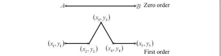
In the early stages ofC. elgansembryogenesis, the zygote (P0) divides into two daugh-ter cells called the andaugh-terior blastomere (AB) and the posdaugh-terior blastomere (P1) forming a 2-cell stage embryo. This is followed by a second round of mitosis, where AB divides into ABa (anterior) and ABp (posterior), while P1 divides into P2 and EMS forming a 4-cell stage embryo (see Figure 1). ABp differentiates into different types of cells including neurons, body muscle, excretory duct cell and hypodermis, while EMS differ-entiates into 42 body muscles and intestine [63]. During organogenesis of the C. ele-gans embryo, ABp differentiates into a nervous system and epidermis, while EMS differentiates into muscular tissues, midgut and pharynx [64]. Axis determination is one of the most important events in the early stages ofC. elegans embryogenesis; as the pronucleus breaks down in the zygote, asymmetric division follows forming a large daughter cell (AB) and a smaller one (P1) establishing the first antero-posterior axis.
AB starts the next division, which is initially oriented orthogonally to the antero-pos-terior axis, but as the cell progresses through anaphase, the orientation of the mitotic spindle of the dividing cell skews, resulting in anterior position of ABa to ABp. P1 commences mitosis a few minutes later resulting in a large EMS progeny cell ventrally located, and a smaller P2 posteriorly located; this round of cell division establishes the dorso-ventral axis [65]. The other important event is garstulation, which begins at the 28-cell stage of development, where Ea and Ep move to the center of the developing embryo and gastrulate forming the three germ layers [64].
There are several reasons for comparing Abp-derived cells (ABp-dc) with those from EMS (EMS-dc). At the developmental level, ABp is derived from the AB blastomere while EMS is derived from the P1 blastomere [66], so ABp and EMS are two different lineages and the use of their cells is relevant in developmental biology. At the organo-genesis level, ABp differentiates into nervous system and epidermis, while EMS differ-entiates into muscular tissue, midgut and pharynx [64], thus ABp and EMS form entirely different organs. At the cellular level, the cells derived from AB blastomere (ABa and ABp) enter the mitotic cycle and divide earlier than those of P1 (EMS and P2), while EMS enters the mitotic cycle earlier than P2 [67]. In addition, ABa and P2 align on the long axis (defining the anterior-posterior poles), while ABp and EMS align on the short axis (defining the dorsal-ventral poles) [68]. Therefore, from temporal and geometrical viewpoints, the derivatives of ABp and EMS are closer to each other, so a more powerful quantitative tool is needed to evaluate their development. At the mole-cular level, P2 is reported to induce polarization in ABp and EMS using MOM-2/Wnt signaling by direct contact between the cells [69].
Experimental setting
The C. elegansdata were obtained according to the previous report of Tiraihi and Tir-aihi [70]. Briefly, aC. elegansembryo (from the 4-cell to the 80-cell stages) was consid-ered, the Cartesian coordinates (x,y,z) were estimated from ABp and EMS cell lineages using the images obtained from SIMI-Biocell [71] and Angler softwares [72]. The Car-tesian coordinates were entered into a computer program to calculate the distances between the cells.
The distances at 30, 55, 82, 109 and 123 minute intervals (fixed intervals) were used at different scales and the data were entered into a computer program used to calcu-late the zero centro-axial skew-symmetrical (CSSM) and the basic square matrices (BSM).
Straight line
Koch curve
The zero order Koch curve is a line comprising two points at the beginning and end, which are named “initiator points”. In order to generate a higher order Koch curve, every line segment was divided into three equal segments. We named the first and the third segments “resting segments”and the second a “generating segment”. The resting segments stay unmodified, and as the name implies, generation takes place in the gen-erating segment. For each line, if we build an equilateral triangle on the gengen-erating seg-ment, the two new lines are called “generated segments”. As the final step in generating the next order, we remove the generating segment(s).
In order to generate a CSSM, we need a set of Cartesian coordinates as the input. For every Koch curve, we consider the end points of every line segment. Before the generation of a higher order curve, the current points satisfying this criterion are called
“resting points”. After the generation, the newly generated points that satisfy this cri-terion are called “generated points”. The ends of each line segment at a certain order are called that order’s principal points.
The algorithm for generating a CSSM from a set of points was described earlier. The initiator line has two principal points, while the 1stand 2ndorder Koch curve have 5 and 17 points, respectively.
A computer program was developed to generate the two-dimensional Cartesian coor-dinates of the points (as described above) of a Koch curve. In this program, the Table 1 The box counting method data used in estimating the scale-invariant power law coefficient of the straight line.
Number of box (NB) Logarithm (NB) Step (h) 1/h Logarithm (1/h)
1 0 48 0.020833333 -1.681241237
2 0.301029996 24 0.041666667 -1.380211242
4 0.602059991 12 0.083333333 -1.079181246
8 0.903089987 6 0.166666667 -0.77815125
16 1.204119983 3 0.333333333 -0.477121255
The box number (NB) and the steps (h) as well as the logarithm of NB and the logarithm of the inverse of step are presented. These data are plotted in figure 1, and the coefficients of the regression line were estimated in order to calculate the SIPL coefficient.
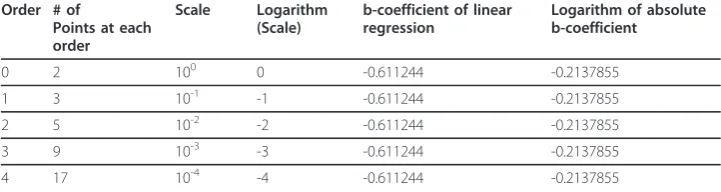
Table 2 The straight line orders and the related parameters used in calculating the scale-invariant power law coefficient using CSSM.
Order # of
Points at each order
Scale Logarithm
(Scale)
b-coefficient of linear regression
Logarithm of absolute b-coefficient
0 2 100 0 -0.611244 -0.2137855
1 3 10-1 -1 -0.611244 -0.2137855
2 5 10-2 -2 -0.611244 -0.2137855
3 9 10-3 -3 -0.611244 -0.2137855
4 17 10-4 -4 -0.611244 -0.2137855
The orders, principal points and scales used in calculating the scale-invariant power law coefficient of the straight line using the zero-centro-axial skew-symmetrical matrix method and the b-coefficients of the regression lines are presented in this table. The data are plotted between the logarithms of the nth root of the absolute value of the basic square
matrix at the order (where n is the number of principal points)
logn
det(BSMorder)
initiator line was a horizontal line of unit length, with the leftmost point (A) located at the origin and the rightmost point (B) at coordinates (1,0) (see Figure 2).
We can also scale the coordinate; for example the line is defined as (A(0,0),B(1,0))) at scale 100and (A(0,0),B(101,0))),(A(0,0,B(102,0))), (A(0,0,B(103,0))) (A(0,0,B(104,0))) (A(0,0,B(105,0))) and (A(0,0, B(106,0))) at scales 10-1, 10-2, 10-3, 10-4, 10-5and 10-6, respectively.
The program calculated the components of the Cartesian coordinates of the princi-pal points for the five orders at different selected scales. These principrinci-pal points were entered into another algorithm in order to generate the zero centro-axial skew-sym-metrical matrix (CSSM) and construct the basic square matrix (BSM) according to the method described in the appendix. The program calculated the two-dimensional Cartesian coordinates (x,y) at the different orders. In the first order (see Figure 2), the program calculated 5 principal points as (1 × n) matrices, hence there were five elements for the x (x1,x2, x3,x4, x5) and y (y1,y2,y3,y4, y5) components. These (1 ×
n) matrices (principal row) were used to generate 5 × 5 CSSMs and 5 × 5 BSMs. In the same way, for the other orders, the principal points of Koch curve were calcu-lated and the principal rows and CSSMs were generated and the BSMs were con-structed. If there were identical elements in the principal row, then one element would be included in the principal row and the others omitted, otherwise the con-structed BSM of the generated CSSM would result in a singular matrix with zero determinant.
For example, for the first order matrix, the program calculated 5 principal points forming two (1 ×n) matrices with 5 elements for each coordinate. This was also done for all the scales in the first order.
The data from the x-components of the Cartesian coordinates of the principal points (A,B) at zero order (initiator) of the Koch curve at 100scale are (A(0,0),B(1,0))), the x-component of the initiator is [(xa,xb) = (0,1)] and the y-component is [(ya, yb) = (0,0)].
If(xa,xb) are considered as the elements of the (1,n) matrix, then the first row of this
matrix is 0[1]. This was used to generate the CSSM for the x-components(xa):
xa=
0 1
−1 0
where a stands for anti-symmetric.
The basic square matrix was constructed according to the algorithm presented in the appendix:
xBSM=
0 4 2 0
The determinant of this matrix is -8.
For the y coordinates,ya= 0 andyBSM= 0, the determinant ofyBSMis zero.
Another CSSM was generated from the combined determinants of xBSMand yBSM; the input elements for the construction of this CSSM were (-8,0). It was translated to the point of origin to construct the CSSM; the principal row was [0,8]. The resulting matrix was:
xycombined=
0 8
−8 0
And the resulting basic square matrix was:
xycombinedBSM =
0 32 16 0
The determinant of the basic square matrix (det(xycombinedBSM)) was -512, this value
represents the determinant of the BSM at Koch curve segment level.
Five orders were used in the study (0th, 1st, 2nd, 3rdand 4th), where the 0thorder is the initiator of Koch curve (straight line). Seven scales (100, 10-1, 10-2, 10-3, 10-4, 10-5 and 10-6) were used in the calculations. At each scale, the determinant of
(xycombinedBSM) was calculated.
Two main operations were involved in calculating the SIPL coefficient; the first was at the order level whereCSSMorderwas used for subsequent calculations, while the sec-ond was at the scale level where linear regression was done in both. The first operation was subdivided into 3 sub-operations. In the first, an iterated algorithm was applied in order to generate CSSMorderand construct BSMorder. For the first order (see Figure 2), the determinant of (xycombinedBSM) of the 0
th
order was used as the first element of this
matrix det(xycombinedBSM(0)) and the second element was the determinant of the first
order det(xycombinedBSM(1)). Then the (1, n) of the first order to generate was
(det(xycombinedBSM(0)), det(xycombinedBSM(1))). This was translated and used in generating
CSSMorder(1), then BSMorder(1) was constructed and its determinant det(BSMorder(1))
was calculated. Similarly, for the second order, the (1, n) matrix was (det(xycombinedBSM(0)), det(xycombinedBSM(1)), det(xycombinedBSM(2))), which was used in
generating CSSMorder(2), constructing BSMorder(2) and calculating det(BSMorder(2)).
For the third and fourth orders (CSSMorder(3) and CSSMorder(4)), the (1, n)
matrices were (det(xycombinedBSM(0)), det(xycombinedBSM(1)), det(xycombinedBSM(2)), det(xycombinedBSM(3))) and (det(xycombinedBSM(0)), det(xycombinedBSM(1)), det(xycombinedBSM(2)), det(xycombinedBSM(3), det(xycombinedBSM(4))), respectively. ThenBSMorder(3)
and BSMorder(4) were constructed and their determinants, det(BSMorder(3)) and det
(BSMorder(4)) were calculated. For the 0th order, det xycombined(0)
was used for
det(BSMorder(0)). In the second sub-operation, the nth root of the absolute value of
BSMorder
n
initiator) was calculated. The calculations were repeated for all the scales (see table 1). In the third sub-operation, for a given scale, the data from the different orders at each scale were plotted using a log-log plot, where the abscissa was the logarithm of the inverse value of step (h) (log(1/h)), while the ordinate was the logarithm of the
abso-lute value ofn
det(BSMorder)
logn
det(BSMorder)
. The log-log plot was fitted for linear regression and the b coefficients for the scales (bscale) were subsequently used in estimating the SIPL of the Koch curve.
For the next operation (scale level), the logarithm of the scale (log(scale)) was plotted against the logarithm of the absolute bscale and another linear regression was calcu-lated. The b coefficient(bSIPL) was used in order to estimate the SIPL according to this equation:SIPL= 1- (D), whereSIPLis the scale-invariant power law coefficient, andD
is bSIPL.
Assessment of validity
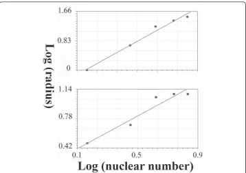
The diffusion-limited aggregate method was used to estimate the fractal dimension of the growing embryo according to Moatamed et al. [73]. Briefly, 5 concentric circles with 5μm increments were superimposed on the center of gravity of ABp-derived cells (ABp-dc) and EMS-derived cells (EMS-dc) at the 123 min. stage of development, and the nuclei of the ABp-derived cells were counted within each circle. The log of the nuclear number was plotted against the log of circle radius, and the slope of the regression line was used as the value of the fractal dimension. The same procedure was done on EMS-dc.
Programming languages
A computer program was written in the C++ language and a text file was generated containing the basic square matrix, which was copied into the command of the matrix of MATLAB® software (http://www.mathworks.com: MathWorks, Inc, Natick, Massa-chusetts) and its determinant was calculated. Also, at each scale (100, 10-1, 10-2, 10-3, 10-4, 10-5and 10-6), the determinants of the basic square matrices were calculated for the following Koch curve orders (0, 1, 2, 3 and 4). The step for each order was also estimated and entered into the calculations.
Results
Straight line
The results for the straight line using the box counting method are presented in detail in table 1 while Figure 3 presents Richardson’s plot; the slope of the regression line equals zero and the SIPL coefficient is one. Table 2 presents the data and the calcula-tions for the straight line using the CSSM. It shows the 4 orders and the number of points at each order, the b coefficients of the linear regression at each order with dif-ferent scales, the logarithm of the absolute value of b coefficients and the scales used for calculating the second regression line in order to estimate the SIPL using the b coefficients (D).
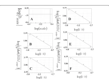
Figure 3Calculations of the scale-invariant power law coefficient of the straight line using the box counting method. The latter is presented using Richardson’s plot logarithm of the inverse of the steps plotted against the logarithm of the box numbers. The regression line has a slope equal to one (y = 1.7 + x: standard error = 0, correlation coefficient = 1).
Figure 4Calculations of the scale-invariant power law coefficient of the straight line using the CSSM method; linear regressions were used to evaluate the straight line. A: presents the logarithms of the scales (log(scale)) plotted against the logarithms of the absolute values of the b coefficients (log| bscale) in the regression line for the data plotted in this figure (B, C, D, E and F). The regression line has a slope equal to zero (y = -0.61: standard error = 0, correlation coefficient = 0.2). The linear regression of the logarithm of the inverse of the steps (log(1/h)) is plotted against the logarithm of the roots of the number of the points on the straight line to the absolute value of the determinant of the basic square matrix
logndet(BSM
order)
10-3 and 10-4, respectively. The abscissa represents the logarithm of the inverse of the
steps plotted againstlogn
det(BSMorder)
(ordinate). In each plot, the 0th, 1st, 2nd, 3rd and 4thorders were entered in order to calculate the linear regression. The logarithms of the absolute values of the b coefficients of the above plots were used for estimating the SIPL of the straight line, which were plotted (ordinate) against the logarithm of the scales (abscissa). The SIPL was calculated as follows: SIPL= 1- (D), where (D) is the b coefficient of the regression line.
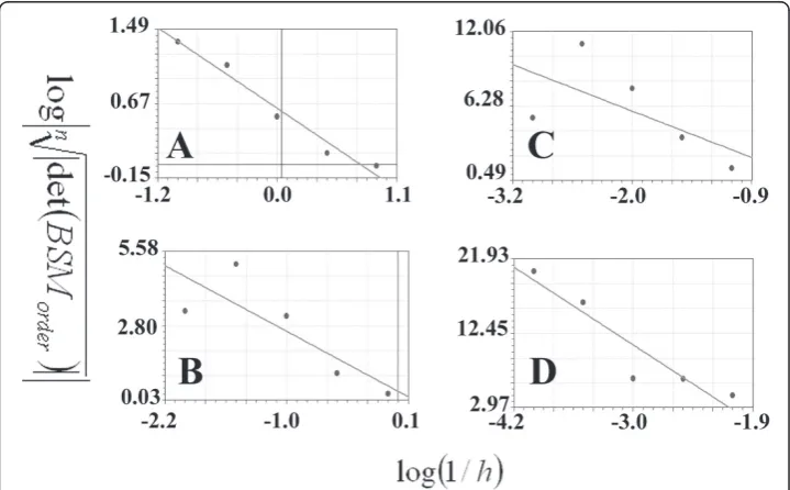
Koch curve
Figure 5 presents the first set of the linear regression of the Koch curve at different scales. There are 4 plots (A, B, C and D) related to 100,10-1, 10-2 and 10-3; three other plots are presented in (Figure 6A, B and 6C) representing the 10-4, 10-5and 10-6scales, respectively. The abscissa presents the logarithms of inverse of the steps (log(1/h))
which were plotted againstlogn
det(BSMorder)
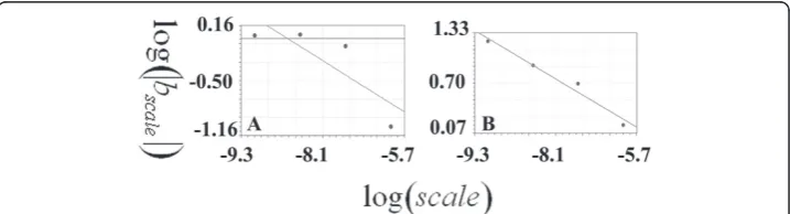
(ordinate). In each plot, the 0th, 1st, 2nd, 3rd and 4thorders were entered in order to calculate the linear regression; the b coefficients are presented in table 3. Figure 6-D presents the plot used for calculating the SIPL (SIPL) of the Koch curve, where the logarithms of the absolute values of the b coefficients(log|bscale|) of the above plots are plotted against the logarithms of the scales (log(scale)). The slope of the regression line was -0.25994438, while the SIPL
Figure 5Calculations of the scale-invariant power law coefficient of the Koch curve using the CSSM method. The linear regression of the logarithm of the inverse of the steps (log(1/h)) is plotted against the logarithm of the roots of the number of the points on the Koch curve to the absolute value of
the determinant of the basic square matrix
logn
det(BSMorder)
. Plot A: presents scale 1 (100), where
Figure 6Calculations of the scale-invariant power law coefficient of the Koch curve using the CSSM method. The linear regression of the logarithm of the inverse of the steps (log(1/h)) is plotted against the logarithm of the root of the number of the points on the Koch curve to the absolute value of
the determinant of the basic square matrix
logndet(BSM
order)
. Plot A: presents scale 4 (10-4) where the 0th, 1st, 2nd, 3rdand 4thorders consist of 2, 5, 17, 65, 257 and 1025 points, respectively. B and C present the other two scales: 10-5and 10-6. The linear regression analyses of the plots are as follows: y = -41.44-15.187x (standard error = 2.36, correlation coefficient = 0.98), y = -73.81-19.81x (standard error = 5.02, correlation coefficient = 0.96), y = -134.43-27.77x (standard error = 5.45 and correlation coefficient = 0.98) for the A, B and C plots. D: presents the logarithms of the scales (log(scale)) plotted against the logarithms of the absolute values of the b coefficients (log|bscale|) in the regression line for the data plotted in figure 3 (A, B, C and D). The regression line has a slope equal to zero as it is presented in a linear regression (y = 0.017-0.26x: standard error = 0.12, correlation coefficient = 0.98).
Table 3 Koch curve orders and the related parameters used in calculating the scale-invariant power law coefficient using CSSM.
Order # of Points at each order
Scale Logarithm (Scale)
b-coefficient of linear regression
Logarithm of absolute b-coefficient
0 2 10-1 -1 -2.1323166 0.328851688
1 5 10-2 -2 -3.1527369 0.49868773
2 17 10-3 -3 -8.6691842 0.937978231
3 65 10-4 -4 -15.187111 1.181475167
4 257 10-5 -5 -19.809067 1.296864021
5 1025 10-6 -6 -27.767092 1.44353039
The number of the orders, principal points and scales used in calculating the SIPL coefficient of the Koch curve using the zero centro-axial skew-symmetrical matrix method and the b-coefficients of the regression lines are presented in this table. The data are plotted between the logarithms of the nth root of the absolute value of the basic square matrix at
the order (where n is the number of principal points)
logn
det(BSMorder)
was 1.25994438 calculated according to the equation SIPL = 1- (D). The analytical fractal value deviation from that was -0.15177%.
Diffusion-limited aggregation
The fractal dimension of ABp-dc was 2.24 (standard error = 0.094; correlation cient = 0.99), and that of EMS-dc was 0.96 (standard error = 0.084; correlation coeffi-cient = 0.96) (see Figure 7).
Developing embryo
The SIPL coefficients were 1.34176236 and 1.33912941 in ABp-dc and EMS-dc, respectively; the regression line of the plotted data is presented in Figure 8.
Discussion
The primary data used in the fractal analysis of the morphological studies are the lengths of the boundaries of the structure, which become more irregular with the increase of scale or magnification [74]. In this study, the components of the Carte-sian coordinates were used as the primary data in the calculation of the SIPL coeffi-cient. The development of an embryo from a fertilized egg is a dynamic process with space and time domains [75]. The spatio-temporal dynamics in developing embryos have studied by several investigators; for example, Wu et al. evaluated fetal develop-ment by plotting the fractal dimension of the brain surface at different stages of development against the time of brain development (in weeks) [76], and a similar approach was used by Schaffner and Ghesquiere in evaluating the complexity of type 1 astrotrocytes using the changes in the fractal dimensions during in vitro differen-tiation of the cells against the time of cell culture [77]. A different approach was taken to evaluating the changes in the value of the fractal dimension using it as a function of time [78]. While self-similarity is a property of fractals [79], cells in the developing C. elegans embryo migrate in a defined direction, becoming located in specific positions as they move. At each stage, the position of each cells is entirely different from the preceding and succeeding stages [70], so self-similarity does not hold during the development of the ABp and EMS sublineages of the C. elegans
embryo. Fractal analysis was used in this study in order to confirm only the power law property of the SIPL, not self-similarity.
The straight line and Koch curve
The SIPL coefficient of the straight line using this method was equal to the fractal dimension using the box counting method, which is consistent with the analytical value of the fractal dimension. The standard error of this regression line was zero. The SIPL of the Koch curve was 1.25994438 with standard error and correlation coefficient equal to 0.1214845 and 0.9810513, respectively. The deviation from the analytical frac-tal dimension value was -0.15177%. The box counting method was reported to be the most suitable and appropriate of the methods discussed by Mandelbrot for estimating the fractal dimension [80] and it is the most popular one [81]. The criterion for select-ing the method is based on the consistency of the fractal dimensions of the straight line and Koch curve. Mola et al. used the box counting method to estimate the fractal dimension of a Koch curve [82], and the results deviated by 2%. Applying the box counting method in calculating the fractal dimension using the fractal dimension cal-culator [83] resulted in a deviation from its analytical value of 6%. Cajueiro et al. used an isometric grid and the result deviated by 0.25% from the analytical fractal value [84]. Jiang et al. also used the box counting method and reported that 3, 4 and 5 recur-sive calculations of the Koch curve resulted in fractal values of 1.212, 1.226 and 1.255 (3.8, 2.6 and 0.4% deviation from the analytical value: 1.26) [85], respectively. There-fore, the consistency of the SIPL coefficient with the fractal dimension suggests the power law property of SIPL. Moreover, a few studies have used the Cartesian coordi-nates as the primary data set in calculating the fractal dimension [86,87], and reported it to be difficult [88], though the use of Cartesian coordinates in field of morphogenesis
has been reported [89]. Also, the application of different methods of fractal dimensions in spatial classification has been considered useful [44], but in the development of the embryo, the spatio-temporal events are more essential for dynamic studies [70].
Diffusion-limited aggregation (DLA)
While diffusion-limited aggregation is used to study aggregation in clusters of particles in the time domain [79], morphogenesis in the developing embryo was studied using the DLA model, which confirmed the fractal property of the developing embryo [90]. DLA was suggested for quantifying the fractal dimension of blood vessel formation in the developing embryo [91] and other branching systems [92]. Therefore, it was used in this study in order to compare it with SIPL in the developing embryo. DLA was also used in the analysis of tumor vasculature [93,94], tumor growth [73,95-99] and in vitro tumor spheroids [100]. The emergence of complex morphology in developing organisms was reported to be caused by DLA [101]. An in vitro study of embryonic retinal neurons showed a decrease in the number of neurite branches with an increase in viscosity of the medium, which was interpreted as a DLA mechanism [102]. Vilela et al. reported that DLA could be used in describing biological growth processes [103]. Therefore, it was used in this study in order to verify the feasibility of using SIPL in the developing embryo.
The developing embryo
A qualitative study was done on self-organization based on the expression of PAR-3, PAR-6 and PKC-3 at the anterior pole of the C. elegans ovum with PAR-1 serine/ threonine kinase and the PAR-2 proteins resulting in anterio-posterior polarization of the embryo [107]; also, there was self-organization at all biological hierarchy levels [1]. In fact, an in vitro study on gastrulation in isolated P1-descendent cells at the 26-cell stage of theC. elegans embryo (tracked in the cultured isolated cells using a 4D video-microscope) showed that the cells gastrulate similarly to those of the intact embryo [108]. Also, a quantitative evaluation of the motion of the isolated cells using an in vitro setting showed that the onset of cellular motion was similar to that in the intact embryo (in vivo) and that the direction of the P1-descendent cells was also similar to that of the in vivo tracked cells [108]. This may indicate that patterning is required for cell population dynamics with the tendency of cells to associate with each other during gastrulation resulting in self-organization [49]. For example, in the vertebrate embryo, vascular patterning is essential for gastrulation movement [109]. On the other hand, in invertebrates, a quantitative study on video microscopy tracked cells at the early stages of C. elegans embryogenesis showed that their motion in the intact embryo was non-random in both EMS and ABp sublineages [70]. In this investigation, we showed that the SIPL coefficient of the EMS lineage is lower than that of the ABp, which is consistent with previous findings about the forward migration index (an index for chemotatic bias) [70]. Therefore, the lower value of the SIPL coefficient is not due to a decline in the complexity [26] or decomplexication of the sublineage [25], but shows that EMS-derived cells start to form an organized structure more rapidly as they tend to regionalize earlier than those of ABp [70]. Tabony documented that self-organization was not related to a single element such as the founder cells in the C. elegansembryo, but arose from the non-linear dynamics of all the elements col-lectively coupled to each other [110]. Schulze and Schierenberg revealed that embryo-nic cell lineages of low complexity formed a single sublineage or generated a single tissue type [111], as in the case of the E cell (from the EMS sublineage). Also, Quin-tana et al. reported that the isolated cells should adhere to each other in order to form an organized structure and suggested that a similar mechanism operated during the early stages of embryogenesis [12].
The results of this investigation are consistent with previous calculations of the diffusion coefficient, a physical parameter reported in a previous communication to be lower in the EMS lineage than in ABp during the early stages of embryogenesis in C. elegans [70]. Moskal and Payatakes reported that a decrease in the fractal dimension indicated a reduction in the diffusion coefficient, so the lower scale-invariant power law coefficient in the EMS lineage may indicate an overall slower motion of EMS-derived than Abp-derived cells. A reduction in the fractal dimension indicates a reduction in the Brownian diffusion coefficient [112], which possesses a random walk property [113], so the results indicate that ABp cells moved more ran-domly than those of EMS.
Conclusion
The study demonstrates that self-organization takes place during the early stages of embryogenesis, as confirmed by a scale-invariant power law method, calculated by using a centro-axial skew symmetrical matrix. The latter was generated from the components of the Cartesian coordinates. The SIPL coefficient results are consistent with DLA, where the fd calculated by DLA indicated that the cells in ABp-dc behaved similarly to type 1 cluster formation, while in EMS-dc they behaved similarly to that of type 2.
Appendix
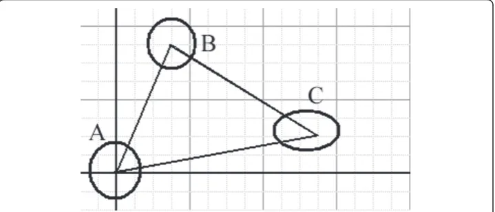
The model used for evaluating the methodology has three points; each was assumed to be a center of gravity of a nucleus of a cell with two neighboring cells. The Cartesian coordinates of the cells were taken in two dimensions and the point of origin of the Cartesian coordinates was translated sequentially to the centers of gravity of all the cells. The x-and y-coordinates of the three cells were used for generating a(3 × 3) zero centro-axial skew-symmetric square matrix (CSSM). Another matrix, a basic square matrix (BSM), was constructed by multiplying the negative elements of the skew matrix with the negative operator (-1), while the positive elements were multiplied by the positive operator (+2). Then all the elements were multiplied by a scalar operator (+2) and the determinants of the matrices were calculated using Matlab software http://www.mathworks.com.
CSSM generation
There are two algorithms for generating CSSM. The first algorithm was accomplished according to the model shown in Figure 9. The nuclei of the three cells (A, B, C) can be seen. There are three states of translating the origin of the Cartesian coordinates (0, 0) to the center of the gravity of each cell:
State 1:
The origin of the Cartesian coordinates is located at the center of nucleus A, and the values of the coordinates for the cells are as follows:
The set of cells is (A, B, C) and the Cartesian coordinates are [(0, 0), (3, 7), (11, 2)]
State 2:
If we translate the origin of the Cartesian coordinates to the center of gravity of cell B, the values will be as follows:
The set of cells is (A, B, C) and the Cartesian coordinates are [(-3, -7), (0, 0), (8, -5)]
State 3:
Likewise for cell C:
The set of cells is (A, B, C) and the Cartesian coordinates are [(-11, -2), (-8, 5), (0, 0)]
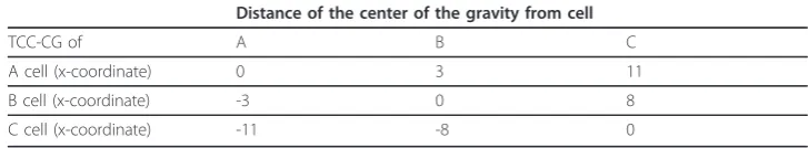
Table 4 presents the arrangement of the x-components, while table 5 presents the y-components for the cells A, B and C in the three states. The array of numbers in table 4 can be presented in this skew matrix, which represents the x-component of the Cartesian coordinates of the centers of gravity of the nuclei in A, B and C cells:
y= ⎡
⎣−0 7 27 0−5
−2 5 0
⎤ ⎦
Similarly, the array of the y-components in table 5 is presented in the following skew matrix:
xycssmcombined=
0 −9312
9312 0
This is a zero centro-axial skew-symmetrical matrix (CSSM).
The second algorithm for CSSM generation was done as described in the methods section. Initially, (1 × 3) matrices for the x-and the y-components [(0,3,11) and (0,7,2), respectively] were used for generating the skew matrices. The CSSM were generated:
xi,j=xi−1,j−xi−1,i (1)
yi,j=yi−1,j−yi−1,i (2)
Where iandjare indices for rows and columns, respectively.
In Euclidean space, the formula can be generalized into n-dimensional space where n = 1, 2, 3, 4...N, and N is a finite number.
xni,j =xn1−1,j−xni−1,i (3)
Table 4 The array of the x-coordinates of the three states of translation for the three cells.
Distance of the center of the gravity from cell
TCC-CG of A B C
A cell (x-coordinate) 0 3 11
B cell (x-coordinate) -3 0 8
C cell (x-coordinate) -11 -8 0
According to Hadley’s [114] notation, the skew symmetric matrices can be rewritten as follows:
xa=
⎡
⎣−03 0 83 11
−11−8 0 ⎤ ⎦
and
ya= ⎡
⎣−0 7 27 0−5
−2 5 0
⎤ ⎦
where the“a”subscript stands for anti-symmetric. 2-Construction of the basic square matrix
The basic square matrices (BSM)xBSMand yBSMwere constructed by multiplying the negative elements of the CSSM by operator (-2) and the positive element by (+4):
xBSM=
⎡
⎣ 0 12 446 0 32 22 16 0
⎤ ⎦
and
yBSM= ⎡
⎣14 0 100 28 8 4 20 0
⎤ ⎦
The determinants of the basic square matrices (and det(yBSM)) were 12672 and 3360, respectively.
A 2 × 2 CSSM can be generated from the values of det(yBSM) by arranging them into
a (1 × 2) matrix in the form of [det(xBSM), det(yBSM)]. This matrix will then be input to the CSSM generation routine and a BSM will be constructed from the CSSM.
For example, for the above values, the input matrix to the CSSM generation process (as described above) will be [12672, 3360] and the CSSM will be (see table 6):
xyCSSMcombined =
0 −9312
9312 0
and the BSM Matrix will be:
xyCSSMcombined =
0 18624
37248 0
Table 5 The array of the y-coordinates of the three states of translation for the three cells.
Distance of the center of the gravity from cell
TCC-CG of A B C
A cell (y-coordinate) 0 7 2
B cell (y-coordinate) -7 0 -5
C cell (y-coordinate) -2 5 0
Finally, the determinant of this matrix is -693706752.
List of abbreviations used
BSM: basic square matrix; CSSM: zero centro-axial skew-symmetrical matrix; dc: descendent cells, derived cells; det: determinant of a matrix; DLA: diffusion-limited aggregation; fd: fractal dimension; SIPL: scale-invariant power law.
Acknowledgements
We would like to express our profound thanks and gratitude to: Professor Dr. Ralf Schnabel (Institut fur Genetik, Technical University at Braunschweig, Germany), who provided the SIMI-BioCell software http://www.simi.com, and The Welcome Trust Sanger Institute at Cambridge. Our gratitude should be extended to other investigators involved in the development of both softwares, and to Mrs. H. AliAkbar for editing the manuscript. We would like to extend my thanks to Dr. Seyed Ahmad Moussavi (Department of Pure Mathematics, Faculty of Mathematical Sciences, Tarbiat Modares University) and Dr Amir Hussein Abbasi (Department of Physics, Faculty of Basic Sciences, Tarbiat Modares University). The project is a self-funded investigation.
Author details 1
College of Computer and Electrical Engineering, Shaheed Behshti University, Tehran, Iran.2Department of Computer Engineering, Sharif University of Technology, Tehran, Iran.3Department of Anatomical Sciences, Faculty of Medical Sciences, Tarbiat Modares University, Tehran, Iran.
Authors’contributions
MT developed the software for generating the data of the components of the Cartesian coordinates and developed the computational techniques in the study, AT contributed to the data analysis and other calculations, and to the writing and organization of the paper. TT developed the theoretical framework, proposed computational techniques, guided the study and led the writing and organization of the paper. All authors read and approved the final manuscript.
Competing interests
The authors declare that they have no competing interests.
Received: 3 September 2010 Accepted: 3 June 2011 Published: 3 June 2011
References
1. Halley JD, Winkler DA:Critical-like self-organization and natural selection: two facets of a single evolutionary process?Biosystems2008,92:148-158.
2. Gerstman BS, Chapagain PP:Self-organization in protein folding and the hydrophobic interaction.J Chem Phys2005, 123:054901.
3. Bagler G, Sinha S:Assortative mixing in Protein Contact Networks and protein folding kinetics.Bioinformatics2007, 23:1760-7.
4. Morra G, Meli M, Colombo G:Molecular dynamics simulations of proteins and peptides: from folding to drug design.Curr Protein Pept Sci2008,9:181-96.
5. Glick BS:Can the Golgi form de novo?Nat Rev Mol Cell Biol2002,3:615-9.
6. Thiele C, Huttner WB:Protein and lipid sorting from the trans-Golgi network to secretory granules-recent developments.Semin Cell Dev Biol1998,9:511-6.
7. Martin W, Russell MJ:On the origins of cells: a hypothesis for the evolutionary transitions from abiotic geochemistry to chemoautotrophic prokaryotes, and from prokaryotes to nucleated cells.Phil Trans R Soc Lond B Biol Sci2003,358(1429):59-83.
8. Kunda P, Baum B:The actin cytoskeleton in spindle assembly and positioning.Trends Cell Biol2009,19:174-9. 9. Guérin T, Prost J, Martin P, Joanny JF:Coordination and collective properties of molecular motors: theory.Curr Opin
Cell Biol2010,22:14-20.
10. Misteli T:The concept of self-organization in cellular architecture.J Cell Biol2001,155:181-5.
11. Maeda TT, Ajioka I, Nakajima K:Computational cell model based on autonomous cell movement regulated by cell-cell signalling successfully recapitulates the“inside and outside”pattern of cell sorting.BMC Syst Biol2007,1:43-59. 12. Quintana L, Muiños TF, Genove E, Del Mar Olmos M, Borrós S, Semino CE:Early tissue patterning recreated by mouse
embryonic fibroblasts in a three-dimensional environment.Tissue Eng Part A2009,15:45-54.
13. Green JB, Dominguez I, Davidson LA:Self-organization of vertebrate mesoderm based on simple boundary conditions.Dev Dyn2004,231:576-81.
Table 6 The (2 × 2) array generated by translation of two points (det(xBSM) and (det (yBSM)) on the real axis to the origin of real axis.
Translation of point on origin of the real axis det(xBSM) det(yBSM)
det(xBSM) 0 -9312
det(yBSM) 9312 0
det(xBSM) is the determinant of the basic square matrix (BSM) constructed from the zero-centro-axial skew-symmetrical matrix (CSSM) presented in table 1.
14. Meinhardt H:Organizer and axes formation as a self-organizing process.Int J Dev Biol2001,45:177-88. 15. ten Berge D, Koole W, Fuerer C, Fish M, Eroglu E, Nusse R:Wnt signaling mediates self-organization and axis
formation in embryoid bodies.Cell Stem Cell2008,3:508-18.
16. Ungrin MD, Joshi C, Nica A, Bauwens C, Zandstra PW:Reproducible, ultra high-throughput formation of multicellular organization from single cell suspension-derived human embryonic stem cell aggregates.PLoS ONE2008,3:e1565. 17. Schiffmann Y:Induction and the Turing-Child field in development.Prog Biophys Mol Biol2005,89:36-92. 18. Su TT:The regulation of cell growth and proliferation during organogenesis.In Vivo2000,14:141-8.
19. Kaneko K, Sato K, Michiue T, Okabayashi K, Danno H, Asashima M:Developmental potential for morphogenesis in vivo and in vitro.J Exp Zool B Mol Dev Evol2008,310:492-503.
20. Wei C, Larsen M, Hoffman MP, Yamada KM:Self-organization and branching morphogenesis of primary salivary epithelial cells.Tissue Eng2007,13:721-35.
21. Schmidt-Ott KM:ROCK inhibition facilitates tissue reconstitution from embryonic kidney cell suspensions.Kidney Int 2010,77:387-9.
22. Beloussov LV, Kazakova NI, Luchinskaia NN, Novoselov VV:Studies in developmental cytomechanic.Int J Dev Biol1997, 41:793-9.
23. Mara A, Holley SA:Oscillators and the emergence of tissue organization during zebra fish somitogenesis.Trends Cell Biol2007,17:593-9.
24. Riedel-Kruse IH, Müller C, Oates AC:Synchrony dynamics during initiation, failure, and rescue of the segmentation clock.Science2007,317(5846):1911-1915.
25. Waliszewski P, Molski M, Konarski J:On the holistic approach in cellular and cancer biology: nonlinearity, complexity, and quasi-determinism of the dynamic cellular network.J Surg Oncol1998,68:70-8.
26. Kurakin A:Scale-free flow of life: on the biology, economics, and physics of the cell.Theor Biol Med Model2009, 6:6-34.
27. Lee S-H, Pak HK, Wi HS, Matsumoto T:Growth dynamics of domain pattern in a three-trophic population model.
Phys A2004,334:233-242.
28. Molski M, Konarski J:Tumor growth in the space-time with temporal fractal dimension.Chaos, Solitons and Fractals 2008,36:811-818.
29. Sawant PD, Nicolau DV:Line and two-dimensional fractal analysis of micrographs obtained by atomic force microscopy of surface-immobilized oligonucleotidenano-aggregates.App Phys Let2005,87:223117-9.
30. Bolliger J, Sprott JC, Mladenoff DJ:Self-organization and complexity in historical landscape patterns.OIKOS2003, 100:541-553.
31. Papageorgiou S, Venieratos D:A reaction-diffusion theory of morphogenesis with inherent pattern invariance under scale variations.J Theor Biol1983,100:57-79.
32. Wearne SL, Rodriguez A, Ehlenberger DB, Rocher AB, Henderson SC, Hof PR:New techniques for imaging, digitization and analysis of three-dimensional neural morphology on multiple scales.Neurosci2005,136:661-80.
33. Gisiger T, Scale invariance in biology:coincidence or footprint of auniversal mechanism?Biol Rev Camb Philos Soc 2001,76:161-209.
34. Pérez MA, Prendergast PJ:Random-walk models of cell dispersal included in mechanobiological simulations of tissue differentiation.J Biomech2007,40:2244-53.
35. Zhang K, Sejnowski TJ:A universal scaling law between gray matter and white matter of cerebral cortex.Proc Natl Acad Sci USA2000,97:5621-6.
36. West GB:The Origin of Universal Scaling Laws in Biology.Physica A1999,263:104-113.
37. West GB, Brown JH, Enquist BJ:The fourth dimension of life: fractal geometry and allometric scaling of organisms.
Science1999,284:1677-1679.
38. Feitzinger JV, Galinski T:The fractal dimension of star-forming in galaxies.Astron Astrophys1987,179:249-254. 39. El Naschie ME:A review of E infinity theory and the mass spectrum of high energy particle physics.Chaos, Solitons
and Fractals2004,19:209-236.
40. Liebovitch LS, Todorov AT:Using fractals and nonlinear dynamics to determine the physical properties of ion channel proteins.Crit Rev Neurobiol1996,10:169-87.
41. Vélez PE, Garreta LE, Martínez E, Díaz N, Amador S, Tischer I, Gutiérrez JM, Moreno PA:The Caenorhabditis elegans genome: a multifractal analysis.Genet Mol Res2010,9:949-65.
42. Mathur SK, Doke AM, Sadana A:Identification of hair cycle-associated genes from time-course gene expression profile using fractal analysis.Int J Bioinform Res Appl2006,2:249-58.
43. Shaw S, Shapshak P:Fractal genomics modeling: a new approach to genomic analysis and biomarker discovery.
Proc IEEE Comput Syst Bioinform Conf2004, 9-18.
44. Jelinek HF, Fernandez E:Neurons and fractals: how reliable and useful are calculations of fractal dimensions?J Neurosci Methods1998,81:9-18.
45. Waliszewski P, Konarski J:Tissue as a self-organizing system with fractal dynamics.Adv Space Res2001,28:545-8. 46. Weibel ER:Fractal geometry: a design principle for living organisms.Am J Physiol1991,261(6 Pt 1):L361-9. 47. Landini G, Misson GP, Murray PI:Fractal analysis of the normal human retinal fluorescein angiogram.Curr Eye Res
1993,12:23-7.
48. Karshafian R, Burns PN, Henkelman MR:Transit time kinetics in ordered and disordered vascular trees.Phys Med Biol 2003,48:3225-37.
49. Phillips CG, Kaye SR:Diameter-based analysis of the branching geometry of four mammalian bronchial trees.Respir Physiol1995,102:303-16.
50. West GB, Woodruff WH, Brown JH:Allometric scaling of metabolic rate from molecules and mitochondria to cells and mammals.Proc Natl Acad Sci USA2002,99(Suppl 1):2473-8.
51. Savage VM, Allen AP, Brown JH, Gillooly JF, Herman AB, Woodruff WH, West GB:Scaling of number, size, and metabolic rate of cells with body size in mammals.Proc Natl Acad Sci USA2007,104:4718-23.
53. Gillooly JF, Charnov EL, West GB, Savage VM, Brown JH:Effects of size and temperature on developmental time.
Nature2002,417(6884):70-3.
54. Gillooly JF, Londoño GA, Allen AP:Energetic constraints on an early developmental stage: a comparative view.Biol Lett2008,4:123-6.
55. Mahmood I:Theoretical versus empirical allometry: Facts behind theories and application to pharmacokinetics.J Pharm Sci2010,99:2927-33.
56. Mahmood I:Evaluation of a morphine maturation model for the prediction of morphine clearance in children: how accurate is the predictive performance of the model?Br J Clin Pharmacol2011,71:88-94.
57. Goteti K, Garner CE, Mahmood I:Prediction of human drug clearance from two species: a comparison of several allometric methods.J Pharm Sci2010,99:1601-13.
58. Grandison S, Morris RJ:Biological pathway kinetic rate constants are scale-invariant.Bioinformatics2008,24:741-3. 59. Ogasawara O, Okubo K:On theoretical models of gene expression evolution with random genetic drift and natural
selection.PLoS One2009,4:e7943.
60. Furusawa C, Kaneko K:Zipf’s Law in Gene Expression.Phys Rev Lett2003,90:088102.
61. Halley JM, Hartley S, Kallimanis AS, Kunin WE, Lennon JJ, Sgardelis SP:Uses and abuses of fractal methodology in ecology.Ecology Lett2004,7:254-271.
62. Milosevic NT, Ristanovic D:Fractal and nonfractal properties of triadic Koch curve.Chaos, Solitons and Fractals2007, 34:1050-1059.
63. Yochem J, Herman RK:InvestigatingC. elegansdevelopment through mosaic analysis.Dev2003,130:4761-8. 64. Labouesse M, Mango SE:Patterning theC. elegansembryo: moving beyond the cell lineage.Trends Genet1999,
15:307-13.
65. Goldstein B, Hird SN, White JG:Cell polarity in earlyC. elegansdevelopment.Dev Suppl1993, 279-87.
66. Irle T, Schierenberg E:Developmental potential of fused Caenorhabditis elegans oocytes: generation of giant and twin embryos.Dev Genes Evol2002,212:257-66.
67. Jaensch S, Decker M, Hyman AA, Myers EW:Automated tracking and analysis of centrosomes in earlyCaenorhabditis elegansembryos.Bioinformatics2010,26:i13-20.
68. Bao Z, Murray JI, Boyle T, Ooi SL, Sandel MJ, Waterston RH:Automated cell lineage tracing inCaenorhabditis elegans.
Proc Natl Acad Sci USA2006,103:2707-12.
69. Bischoff M, Schnabel R:A posterior centre establishes and maintains polarity of theCaenorhabditis elegansembryo by a Wnt-dependent relay mechanism.PLoS Biol2006,4:e396.
70. Tiraihi A, Tiraihi T:Early onset of regionalization in EMS lineage ofC. elegansembryo: a quantitative study.
Biosystems2007,90:676-86.
71. Simi Reality Motion Systems GmbH.[http://www.simi.com].
72. The Welcome Trust Sanger Institute at Cambridge, UK.[http://www.sanger.ac.uk/Software/Angler/].
73. Moatamed F, Sahimi M, Naeim F:Fractal dimension of the bone marrow in metastatic lesions.Hum Pathol1998, 29:1299-303.
74. Gisiger T:Scale invariance in biology: coincidence or footprint of a universal mechanism?Biol Rev Camb Philos Soc 2001,76:161-209.
75. Nottale L:Scale relativity and fractal space-time: theory and applications. In: the evolution and development of the universe.InIn The first international conference on the evolution and development of the universe, 8-9 October 2008, Ecolenormalesupérieure, ParisEdited by: Vidal C 2008, 1-65.
76. Wu YT, Shyu KK, Chen TR, Guo WY:Using three-dimensional fractal dimension to analyze the complexity of fetal cortical surface from magnetic resonance images.Nonlinear Dynamics2009,58:745-752.
77. Schaffner AE, Ghesquiere A:The effect of type 1 astrocytes on neuronal complexity: a fractal analysis.Methods2001, 24:323-329.
78. Parsons-Wingerter P, Elliott KE, Farr AG, Radhakrishnan K, Clark JI, Sage EH:Generational analysis reveals that TGF-beta1 inhibits the rate of angiogenesis in vivo by selective decrease in the number of new vessels.Microvasc Res 2000,59:221-32.
79. Meakin P:Fractal structures.Prog Solid St Chem1990,20:135-233.
80. Foroutan-pour K, Dutilleul P, Smith DL:Advances in the implementation of the box-counting method of fractal dimension estimation.Appl Math Comput1999,105:195-210.
81. Buczkowski S, Kyriacos S, Nekka F, Cartilier L:The modified box-counting method: Analysis of some characteristic parameters.Pattern Recognition1998,31:411-418.
82. Mola MM, Haddad R, Hill S:Fractal flux jumps in the organic superconducting crystal.Solid State Commun2006, 127:611-614.
83. Elert G:The Chaos Hypertextbook™1995-2007[http://hypertextbook.com/chaos/33.shtml].
84. Cajueiro DO, de A Sampaio VA, de Castilho CMC, Andrade RFS:Fractal properties of equipotentials close to a rough conducting surface.J Phys Condens Matter1999,11:4985-4992.
85. Jiang Y, Tanabashi Y, Li B, Xiao J:Influence of geometrical distribution of rock joints on deformational behavior of underground opening.Tunnel Underground Space Technol2006,21:485-491.
86. Costa LdF, Barbosa MS, Manoel ETM, Streicher J, Muller GB:Mathematical characterization of three-dimensional gene expression patterns.Bioinform2004,20:1653-1662.
87. Peng T, Feng Z:The box-counting measure of the star product surface.Intl J Nonlinear Sci2008,6:281-288. 88. Wegman EJ, Solka JL:On some mathematics for visualising high dimensional data.Indian J Statistics2002,64(Series
A, 2):429-452.
89. Goodall N, Kisiswa L, Prashar A, Faulkner S, Tokarczuk P, Singh K, Erichsen JT, Guggenheim J, Halfter W, Wride MA: 3-Dimensional modelling of chick embryo eye development and growth using high resolution magnetic resonance imaging.Exp Eye Res2009,89:511-21.
90. Blazsek I, Innate chaos I:The origin and genesis of complex morphologies and homeotic regulation.Biomed Pharmacother1992,46:219-35.
93. Baish JW, Jain RK:Fractals and cancer.Cancer Res2000,60:3683-8. 94. Baish JW, Jain RK:Cancer, angiogenesis and fractals.Nat Med1998,4:984.
95. Sander LM, Deisboeck TS:Growth patterns of microscopic brain tumors.Phys Rev E Stat Nonlin Soft Matter Phys2002, 66(5 Pt 1):051901.
96. Hatzikirou H, Deutch A:Mathematical modeling of glioblastoma tumor development: a review.Math Mod and MethAppl2005,15:1779-1794.
97. Stein AM, Demuth T, Mobley D, Berens M, Sander LM:A mathematical model of glioblastoma tumor spheroid invasion in a three-dimensional in vitro experiment.Biophys J2007,92:356-65.
98. Flores-Ascencio S, Perez-Meana H, Nakano-Miyatake M:A three dimensional growth model for primary cancer.The Fourth International Kharkov Symposium on Physics and Engineering of Millimeter and Sub-Millimeter Waves: 4-9 June 2001; Kharkov, Ukraine241-243.
99. Dobrescu R, Ichim L, Mocanu S, Popa S:A fractal model for simulation of biological growth processes.9th WSEAS Int. Conf. on Mathematics and Computer in Biology and Chemistry (MCBC 2008): June 24-26, 2008; Bucharest, Romania2008, 88-93.
100. Engelberg JA, Ropella GE, Hunt CA:Essential operating principles for tumorspheroid growth.BMC SystBiol2008, 2:110-119.
101. Blazsek I:Innate chaos: I. The origin and genesis of complex morphologies and homeotic regulation.Biomed Pharmacother1992,46:219-35.
102. Caserta F, Hausman RE, Eldred WD, Kimmel C, Stanley HE:Effect of viscosity on neurite outgrowth and fractal dimension.Neurosci Lett1992,136:198-202.
103. Vilela MJ, Martins ML, Boschetti SR:Fractal patterns for cells in culture.J Pathol1995,177:103-7.
104. Ryabov AB, Postnikov EB, Loskutov AYu:Diffusion-Limited Aggregation: A Continuum Mean Field Model.J Exp Theort Phys2005,101:253-258.
105. Kajiwara K:Structure of gels.InGels handbook.Edited by: Kajiwara K, Osada Y. San Deigo: Academic press; 2001:122-171.
106. Peker SM, HelvacıSS, Yener B,İkizler B, Alp A:The Particulate Phase: A Voyage from the Molecule to the Granule.In Solid-liquid two phase flow.Edited by: Peker SM, HelvacıSS. Amsterdam: Elsevier; 2008:1-70.
107. Zallen JA, Blankenship JT:Multicellular dynamics during epithelial elongation.Semin Cell Dev Biol2008,19:263-270. 108. Lee J-Y, Goldstein B:Mechanisms of cell positioning during C. elegansgastrulation.Dev2003,130:307-320. 109. Fleury V, Unbekandt M, Al-Kilani A, Nguyen TH:The textural aspects of vessel formation during embryo
development and their Relation to gastrulation movements.Organogenesis2007,3:49-56.
110. Tabony J:Historical and conceptual background of self-organization by reactive processes.Biol Cell2006, 98:589-602.
111. Schulze J, Schierenberg E:Embryogenesis of Romanomermisculicivorax: an alternative way to construct a nematode.Dev Biol2009,334:10-21.
112. Moskal A, Payatakes AC:Estimation of the diffusion coefficient of aerosol particle aggregates using Brownian simulation in the continuum regime.Aerosol Sci2006,37:1081-1101.
113. Wong A, Wu L, Gibbons PB, Faloutsos C:Fast estimation of fractal dimension and correlation integral on stream data.Inform Process Let2005,93:91-97.
114. Hadley G:Linear algebraReading: Addison-Wesley; 1961.
doi:10.1186/1742-4682-8-17
Cite this article as:Tiraihiet al.:Self-organization of developing embryo using scale-invariant approach.
Theoretical Biology and Medical Modelling20118:17.
Submit your next manuscript to BioMed Central and take full advantage of:
• Convenient online submission
• Thorough peer review
• No space constraints or color figure charges
• Immediate publication on acceptance
• Inclusion in PubMed, CAS, Scopus and Google Scholar
• Research which is freely available for redistribution