Bootstrap Confidence Intervals of the Difference between Two Process Capability Indices for Half Logistic Distribution

Two Process Capability Indices for Half Logistic Distribution

Wararit Panichkitkosolkul

Department of Mathematics and Statistics Faculty of Science and Technology

Thammasat University, Phathum Thani, Thailand [email protected]

Somchit Wattanachayakul

Department of Mathematics and Statistics Faculty of Science and Technology

Thammasat University, Phathum Thani, Thailand [email protected]

Abstract

The process capability indices are important numerical measures in statistical quality control. Well-known process capability indices are constructed under the process distribution is normal. Unfortunately, this situation is rather not realistic. This paper focuses on the half logistic distribution. The bootstrap confidence intervals for the difference between two process capability indices for the mentioned distribution are proposed. The bootstrap confidence intervals considered in this paper consist of the standard bootstrap confidence interval, the percentile bootstrap confidence interval and the bias-corrected percentile bootstrap confidence interval. A Monte Carlo simulation has been used to investigate the estimated coverage probabilities and average widths of the bootstrap confidence intervals. Simulation results showed that the estimated coverage probabilities of the percentile bootstrap confidence interval and the bias-corrected percentile bootstrap confidence interval get closer to the nominal confidence level than those of the standard bootstrap confidence interval.

Keywords: Process capability index, Bootstrap confidence interval, Half logistic distribution.

1. Introduction

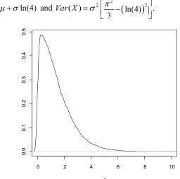
The half logistic distribution, which is the distribution of the absolute logistic random variable, was introduced by Balakrishnan (1985). The main references about the half logistic distribution include Balakrishnan and Chan (1992), Balakrishnan and Wong (1994) and Balakrishnan and Aggarwala (1996). If Y is a logistic random variable, then

X Y has a half logistic distribution. The probability density function ( ( ))f x and the cumulative distribution function ( ( ))F x are









2exp ( ) /

( ) ,

1 exp ( ) /

x f x

x  

  

  

  

 

  (1.1)

and





1 exp ( ) /

( ) x , 0, 0,

the probability density function for half logistic distribution is shown in Fig. 1.1 The mean and the variance of X are defined as

( ) ln(4)

E X    and _{( )} 2 2





3

Var X  _  _

 

Figure 1.1 The probability density function for half logistic distribution with  0 and 1.

 

Several studies have applied the half logistic distribution. For instance, Balakrishnan (1985) has suggested the usage of this distribution as a possible life-time model with an increasing hazard rate. In addition, Balakrishnan and Chan (1992) have shown that the failure times of air conditioning equipment in a Boeing 720 airplane fits the half logistic distribution quite well. This distribution was also applied to environmental and sports records data (Mbah and Tsokos, 2008). In recent papers, many authors have applied the half logistic distribution under progressive Type-II censoring (see Kang et al., 2008, Balakrishnan and Saleh, 2011, Jang et al. 2011). As mentioned above, it is known that the half logistic distribution is an increasing failure rates model with reasonable importance in statistical quality control and reliability studies (see Kantam and Rosaiah 1998,Kantam et al. 2000, Srinivasa, 2004, Satyaprasad, 2007, Rosaiah et al., 2009, Kantam et al., 2010).

One of the statistical quality control tools widely used is the process capability index (PCI). This index uses both process variability and process specification to determine whether the process is capable (Peng, 2010). Even though there are many process capability indices, the two most commonly used indices are Cp and Cpk(Kane, 1986,

Zhang, 2010). In this paper, we focus only on the popular process capability index C_pk

defined as follows

min , ,

3 3

pk USL LSL

C  _{ } _ _ (1.3)

0 2 4 6 8 10

0.

0

0.

1

0.

2

0.

3

0.

4

0.

5

where USL and LSL denote respectively the upper and lower specification limits of the process,  is the process mean and  is the process standard deviation. As the process standard deviation and the process mean are unknown, they must be estimated from the sample data { ,..., }.X1 Xn Under the normality assumption, the sample mean X;

1 1

n i i X n X







1

( 1) n ( i )

i

S n  X X



 



to estimate the unknown parameters  and in Eq. (1.3), respectively. Therefore, the natural estimator of the process capability index Cpk can be obtained as

min , .

3 3

pk USL X X LSL

C

S S

   

 _{ }

 



However, the underlying process distribution is non-normal in some situations. Hence, it may be a skewed distribution. To deal with these phenomena, Clements (1989) proposed a new method for computing the estimator of the process capability index Cpk when the

process distribution is non-normal. This estimator is defined as

min , ,

pk

p p

USL M M LSL C

U M M L

 _{ } 

 

 _{ }

 

 

 



(1.4)

where U Lp, p and M denote the 99.865th percentile, the 0.135th percentile and the 50th

percentile of the distribution, respectively. The advantage of Cpk



shown in Eq.(1.4) is that it can be applied to any distribution. Kantam et al. (2010) discussed the relationship between Cpk



and the probability that a product falling outside the specification limits when X has a half logistic distribution. This probability is given by

( ) ( ) 1 ( ) ( ),

t

P P X LSL P X USL     F LSL F USL

where F( ) is the cumulative distribution function of a half logistic distribution shown in Eq.(1.2). Using the open source statistical package R (Ihaka and Gentleman 1996), some values of L U_p, _p and M for the half logistic distribution are shown in Table 1.

Table 1: The values of L U_p, _p and M for the half logistic distribution

 _{ Lp Up M}

0 1 0.002700002 7.300123 1.098612

0 1.5 0.00405 10.95018 1.647918

0.5 1 0.5027 7.800123 1.598612

0.5 1.5 0.50405 11.45018 2.147918

1 1 1.0027 8.300123 2.098612

The estimator Cpk



in Eq. (1.4) can be applied when the scale parameter  of the half logistic distribution is equal to 1. Therefore, if a scale parameter  is introduced and known, i.e.,  1 _{in Eq.(1.1), the optimal estimator of Cpk is given by}

min , .

( ) ( )

pk

p p

USL M M LSL

C

U M M L

     _{ }      _{ }       

In practice, the scale parameter  is unknown. Therefore, we must estimate the unknown

 by its estimator. In this paper, we use the moment method for calculating this estimator. The estimator of C_pk for a half logistic distribution is

ˆ ˆ

ˆ _{min , ,}

ˆ( ) ˆ( )

pk

p p

USL M M LSL

C

U M M L

     _{ }     _{ }    

  (1.5)

where ˆ is the estimator of . Here, we use the simple estimator which is computed by

the moment method given by ˆ 1 ˆ

ln(4) X

  _ _ and the maximum likelihood estimator

for  is ˆ  X(1), the smallest sample order statistics. The moments of the half logistic

distribution were shown in Giles (2012).

In this paper, our focus is on the difference between two process capability indices,

1 2,

pk pk

C C which we will denote by which

1 1 2 2

1 1 2 2

min , min , ,

3 3 3 3

USL   LSL USL   LSL



   

       

 _{ } _{ }

   

where  1, 2 and  1, 2 are the process mean and standard deviation of the first and the

second population, respectively. Similar to Eq.(1.5), we can get the estimator of  which is

1 1 1 1 2 2 2 2

1 1 1 1 1 1 2 2 2 2 2 2

ˆ ˆ ˆ ˆ

ˆ min , min , ,

ˆ ( p ) ˆ ( p ) ˆ ( p ) ˆ ( p )

USL M M LSL USL M M LSL

U M M L U M M L

          _{ }   _{ }       _{ } _{ }        

    (1.6)

where ˆ1 and ˆ2 are the moment estimator of 1 and 2given by ˆ1 _ln(4)1 X1ˆ1

and ˆ2 _ln(4)1 X2ˆ ,2 respectively, ˆ1 X1(1) and ˆ2 X2(1).

results and conclusions are presented in the final section. The conclusions are offered in the final section.

2. Bootstrap Confidence Intervals

The bootstrap is a computer-based and resampling method for assigning measures of accuracy to statistical estimates (Efron and Tibshirani, 1993). Many types of bootstrap methods for constructing confidence intervals have been introduced; for example, the standard bootstrap method (SB), the percentile bootstrap method (PB) and the bias-corrected percentile bootstrap method (BCPB).

For a sequence of independent and identically distributed (i.i.d.) random variables, the bootstrap procedure can be defined as follows (Tosasukul et al., 2009). Let the random variables {Xk j, ,1 j m} be the result from sampling m times from the kth population

with replacement from the n observations X_k,1,...,X_{k n,} . The random variables

,

{X_{k j} ,1_{ }j m} _{are called the bootstrap samples from original data}

,1,..., , .

k k n

X X In what

follows, we describe the constructions for the confidence interval of the difference between two process capability indices using bootstrap techniques.

2.1 Standard Bootstrap (SB) Confidence Interval

Let Xk b, , where 1 b B, and k1, 2 be the bth bootstrap samples and let Xk,1,...,Xk B,

be the B bootstrap samples. The _bth _{bootstrap estimator of  is computed by}

( ) ( ) ( ) ( )

( ) 1 1 1 1 2 2 2 2

( ) ( ) ( )

1 1 1 1 1 1 2 2 2 2 2 2

ˆ ˆ ˆ ˆ

ˆ _{min , min , ,}

ˆ ( ) ˆ ( ) ˆ ( ) ˆ ( )

b b b b

b

b b b

p p p p

USL M M LSL USL M M LSL

U M M L U M M L

                   _{ }   _{ }       _{ } _{ }        

    (2.1)

where ( ) ( )

1 1

ˆ b _X b / ln(4),

 _  ( ) 1 1

1 1 1,

1 , n b j j X n X







2 2

ˆ b _X b / ln(4),

 _  ( ) 1 2

2 2 2,

1 , n b j j X n X







the standard bootstrap (1)100% confidence interval is

1 1

2 2

ˆ _, ˆ _,

SB Z S Z S

CI   _   _ 

  (2.2)

where Z1/ 2 is a 1/ 2thquantile of the standard normal distribution, 1 ( ) 1

ˆ B ˆ i

i B     







( ) ( ) 1

1 _{ˆ ˆ .}

2.2 Percentile Bootstrap (PB) Confidence Interval

The percentile bootstrap (1)100% confidence interval is given by

1

2 2

ˆ _, ˆ _,

PB B B

CI _ _ _    

    

 

 _ _ (2.3)

where ˆ( )r is the rth ordered value on the list of the B bootstrap estimator of .

2.3 Bias-Corrected Percentile Bootstrap (BCPB) Confidence Interval

The obtained bootstrap distributions using only a sample of the complete bootstrap distribution may be shifted higher or lower than would be expected. Therefore, this approach has been introduced in order to correct for the potential bias. Firstly, using the ordered distribution of ˆ , _{compute the probability}

0 (ˆ ˆ).

P P_ _ _Then, 1

0 ( ).0

Z _{ } P

Therefore, the percentile of the ordered distribution _G*_{( ),}ˆ





0 1 / 2

2

L

P   Z Z  and





U

P   Z Z  are obtained, where  ( ) is the standard normal cumulative

function. Finally, the bias-corrected percentile bootstrap (1)100% confidence interval is defined as follows





BCPB P B P B

CI _   _(2.4)

whereˆ( )r is the rth ordered value on the list of the B bootstrap estimator of .

To study the different confidence intervals, we consider their estimated coverage probabilities and average widths. For each of the methods considered, the probability that the true value of C_pk is covered by the (1)100% bootstrap confidence interval, which is called the “coverage probability”, can be obtained. In addition, the average width of the bootstrap confidence interval is calculated based on the M 5,000different trials .The estimated coverage probability and the average width are given by

 #( )

1 L U ,

M 

  

 

and

 1

( )

,

M

i i i

U L Width

M



 



where L andU denote the lower and upper bound of the bootstrap confidence interval.

In the following section, a simulation study is presented in order to evaluate the performance of the confidence intervals CISB,CIPB, and CIBCPB based on their estimated

3. Simulation Study

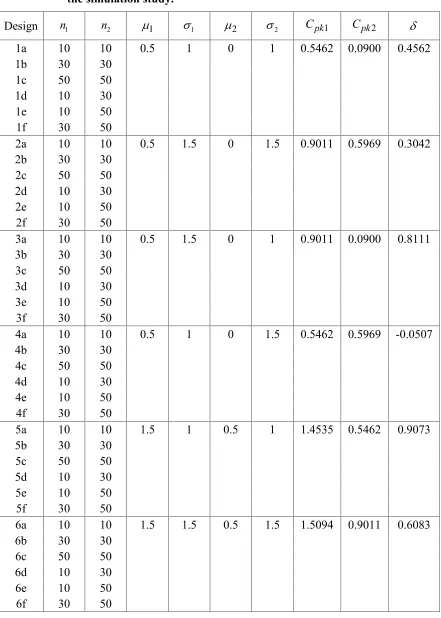
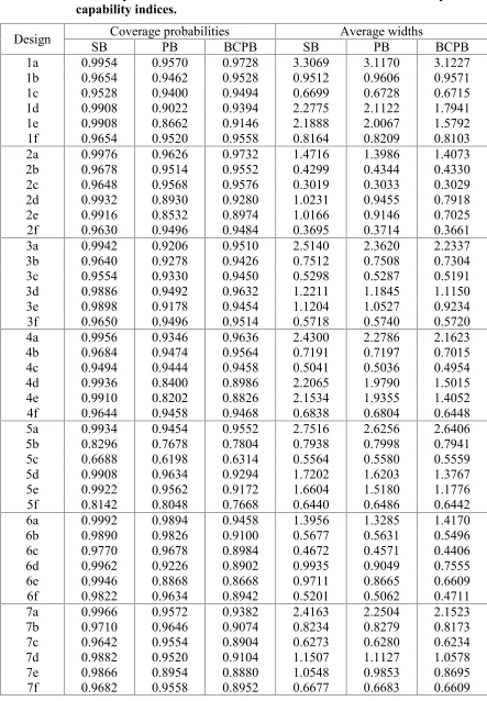
A simulation study on the behavior of three bootstrap confidence intervals of the difference between two process capability indices for half logistic distribution is described. The statistical package R (Ihaka and Gentleman, 1996) is used to carry out the simulation study in this section. In addition, the sample sizes and parameter values of half logistic distribution that we used in this simulation are listed in Table 2. Similar to previous experiments of Kantam et al. (2010), we set the lower and upper specification limits are 1 and 29, respectively. The process capability indices and the difference between the two process capability indices of twelve designs are shown in Table 2. For each design, B1,000 bootstrap samples with each of size n are drawn from the original sample. Additionally, the simulation is replicated 5,000 times. The 90% and 95% bootstrap confidence intervals are constructed by each of the three methods, i.e., SB, PB, and BCPB confidence intervals.

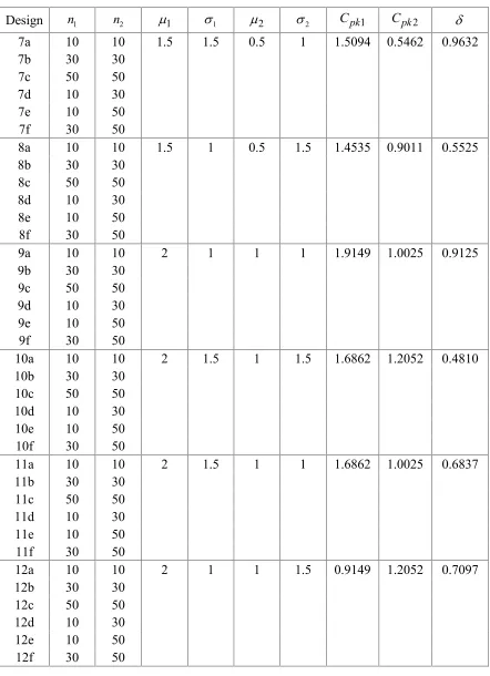
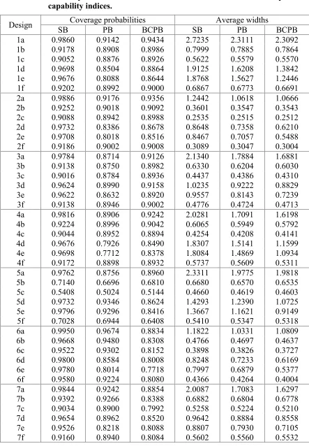
The simulation results are summarized in Tables 3 and 4. These two tables present the results on the estimated coverage probabilities and average widths of 90% and 95% bootstrap confidence intervals, respectively. We begin with the results for Designs 1a-f, 2a-f, 3a-f and 4a-f ( 1 1 and 2 2), the estimated coverage probabilities of CISB

are larger than the nominal confidence level. In addition, the estimated coverage probabilities ofCIBCPBget reasonably closer to the nominal confidence level than those of

SB

CI and CIPB for all sample sizes. When Designs 6a-f and 7a-f ( 1 1 and 2 2)

are considered, the estimated coverage probabilities of CISBare not less than the nominal

confidence level. The CIPB provides the estimated coverage probabilities closer to the

nominal confidence level than those ofCISB and CIBCPB.

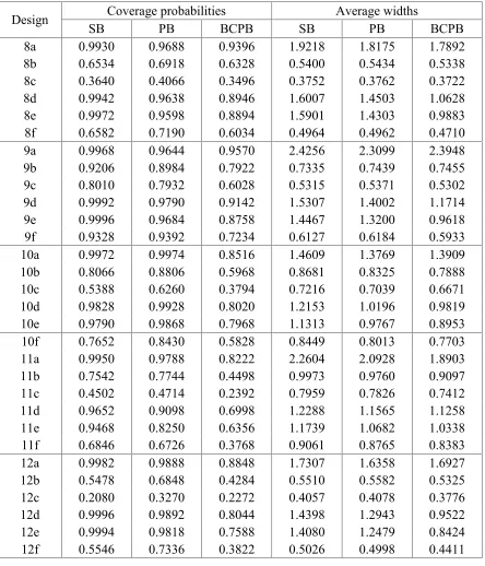
As one can see, under Designs 5a-f, 8a-f, 9a-f, 10a-f, 11a-f and 12a-f ( 1 1 and

2 2

  ), the CISB,CIPB, and CIBCPBgive poor coverage probabilities than the nominal

confidence level for large sample sizes. On the other hand, the estimated coverage probabilities of CISBare significantly above the nominal confidence level for small

sample size (n n1  2 10).

The CIBCPB provides the shortest average width for all situations. Additionally, the

average widths of all the bootstrap confidence intervals get shorter when n₁and (or) n₂

Table 2: Sample sizes and parameter values of half logistic distribution used in the simulation study.

Design n1 n2 1 1 2 2 Cpk1 Cpk2 

1a 10 10 0.5 1 0 1 0.5462 0.0900 0.4562

1b 30 30

1c 50 50

1d 10 30

1e 10 50

1f 30 50

2a 10 10 0.5 1.5 0 1.5 0.9011 0.5969 0.3042

2b 30 30

2c 50 50

2d 10 30

2e 10 50

2f 30 50

3a 10 10 0.5 1.5 0 1 0.9011 0.0900 0.8111

3b 30 30

3c 50 50

3d 10 30

3e 10 50

3f 30 50

4a 10 10 0.5 1 0 1.5 0.5462 0.5969 -0.0507

4b 30 30

4c 50 50

4d 10 30

4e 10 50

4f 30 50

5a 10 10 1.5 1 0.5 1 1.4535 0.5462 0.9073

5b 30 30

5c 50 50

5d 10 30

5e 10 50

5f 30 50

6a 10 10 1.5 1.5 0.5 1.5 1.5094 0.9011 0.6083

6b 30 30

6c 50 50

6d 10 30

6e 10 50

Table 2: (Continued)

Design n1 n2 1 1 2 2 Cpk1 Cpk2 

7a 10 10 1.5 1.5 0.5 1 1.5094 0.5462 0.9632

7b 30 30

7c 50 50

7d 10 30

7e 10 50

7f 30 50

8a 10 10 1.5 1 0.5 1.5 1.4535 0.9011 0.5525

8b 30 30

8c 50 50

8d 10 30

8e 10 50

8f 30 50

9a 10 10 2 1 1 1 1.9149 1.0025 0.9125

9b 30 30

9c 50 50

9d 10 30

9e 10 50

9f 30 50

10a 10 10 2 1.5 1 1.5 1.6862 1.2052 0.4810

10b 30 30

10c 50 50

10d 10 30

10e 10 50

10f 30 50

11a 10 10 2 1.5 1 1 1.6862 1.0025 0.6837

11b 30 30

11c 50 50

11d 10 30

11e 10 50

11f 30 50

12a 10 10 2 1 1 1.5 0.9149 1.2052 0.7097

12b 30 30

12c 50 50

12d 10 30

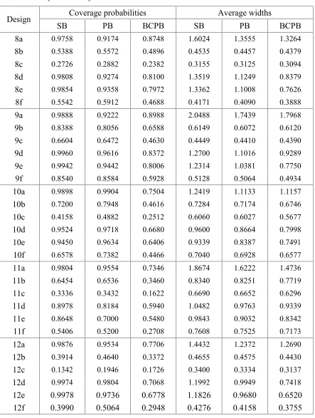
Table 3: The estimated coverage probabilities and average widths of a 90% bootstrap confidence intervals of the difference between two process capability indices.

Design _SBCoverage probabilities_{PB BCPB SB} Average widths_{PB BCPB}

1a 0.9860 0.9142 0.9434 2.7235 2.3111 2.3092

1b 0.9178 0.8908 0.8986 0.7999 0.7885 0.7864

1c 0.9052 0.8876 0.8926 0.5622 0.5579 0.5570

1d 0.9698 0.8504 0.8864 1.9125 1.6208 1.3842

1e 0.9676 0.8088 0.8644 1.8768 1.5627 1.2446

1f 0.9202 0.8992 0.9000 0.6867 0.6773 0.6691

2a 0.9886 0.9176 0.9356 1.2442 1.0618 1.0666

2b 0.9252 0.9018 0.9092 0.3601 0.3547 0.3543

2c 0.9088 0.8942 0.8988 0.2535 0.2515 0.2512

2d 0.9732 0.8386 0.8678 0.8648 0.7358 0.6210

2e 0.9708 0.8018 0.8516 0.8467 0.7057 0.5488

2f 0.9186 0.9002 0.9008 0.3089 0.3047 0.3004

3a 0.9784 0.8714 0.9126 2.1340 1.7884 1.6881

3b 0.9138 0.8750 0.8982 0.6330 0.6204 0.6030

3c 0.9016 0.8784 0.8936 0.4437 0.4386 0.4310

3d 0.9624 0.8990 0.9158 1.0235 0.9222 0.8829

3e 0.9622 0.8632 0.8920 0.9557 0.8143 0.7239

3f 0.9138 0.8946 0.9002 0.4776 0.4724 0.4713

4a 0.9816 0.8906 0.9242 2.0281 1.7091 1.6198

4b 0.9224 0.8996 0.9042 0.6065 0.5949 0.5792

4c 0.9044 0.8952 0.8894 0.4254 0.4208 0.4141

4d 0.9676 0.7926 0.8490 1.8307 1.5141 1.1599

4e 0.9698 0.7712 0.8378 1.8084 1.4869 1.0934

4f 0.9172 0.8898 0.8932 0.5737 0.5609 0.5311

5a 0.9762 0.8756 0.8960 2.3311 1.9775 1.9818

5b 0.7140 0.6696 0.6810 0.6680 0.6570 0.6535

5c 0.5408 0.5024 0.5144 0.4660 0.4619 0.4603

5d 0.9732 0.9346 0.8624 1.4293 1.2390 1.0725

5e 0.9796 0.9296 0.8416 1.3667 1.1621 0.9149

5f 0.7028 0.6944 0.6408 0.5410 0.5347 0.5318

6a 0.9950 0.9674 0.8834 1.1822 1.0331 1.0809

6b 0.9668 0.9480 0.8308 0.4766 0.4697 0.4637

6c 0.9522 0.9302 0.8152 0.3898 0.3826 0.3727

6d 0.9800 0.8584 0.8008 0.8248 0.7233 0.6169

6e 0.9780 0.8014 0.7718 0.7997 0.6879 0.5377

6f 0.9580 0.9224 0.8080 0.4366 0.4264 0.4004

7a 0.9844 0.9242 0.8854 2.0087 1.7083 1.6297

7b 0.9392 0.9266 0.8388 0.6882 0.6804 0.6778

7c 0.9034 0.8900 0.7992 0.5258 0.5224 0.5210

7d 0.9654 0.8962 0.8520 0.9642 0.8884 0.8558

Table 3: (Continued)

Design Coverage probabilities Average widths

SB PB BCPB SB PB BCPB

8a 0.9758 0.9174 0.8748 1.6024 1.3555 1.3264

8b 0.5388 0.5572 0.4896 0.4535 0.4457 0.4379

8c 0.2726 0.2882 0.2382 0.3155 0.3125 0.3094

8d 0.9808 0.9274 0.8100 1.3519 1.1249 0.8379

8e 0.9854 0.9358 0.7972 1.3362 1.1008 0.7626

8f 0.5542 0.5912 0.4688 0.4171 0.4090 0.3888

9a 0.9888 0.9222 0.8988 2.0488 1.7439 1.7968

9b 0.8388 0.8056 0.6588 0.6149 0.6072 0.6120

9c 0.6604 0.6472 0.4630 0.4449 0.4410 0.4390

9d 0.9960 0.9616 0.8372 1.2700 1.1016 0.9289

9e 0.9942 0.9442 0.8006 1.2314 1.0381 0.7750

9f 0.8540 0.8584 0.5928 0.5128 0.5064 0.4934

10a 0.9898 0.9904 0.7504 1.2419 1.1133 1.1157

10b 0.7200 0.7948 0.4616 0.7284 0.7174 0.6746

10c 0.4158 0.4882 0.2512 0.6060 0.6027 0.5677

10d 0.9524 0.9718 0.6680 0.9600 0.8664 0.7998

10e 0.9450 0.9634 0.6406 0.9339 0.8387 0.7491

10f 0.6578 0.7382 0.4466 0.7040 0.6928 0.6577

11a 0.9804 0.9554 0.7346 1.8674 1.6222 1.4736

11b 0.6454 0.6536 0.3460 0.8340 0.8251 0.7719

11c 0.3336 0.3432 0.1622 0.6690 0.6652 0.6296

11d 0.8978 0.8184 0.5940 1.0482 0.9763 0.9339

11e 0.8648 0.7000 0.5480 0.9843 0.9032 0.8342

11f 0.5406 0.5200 0.2708 0.7608 0.7525 0.7173

12a 0.9876 0.9534 0.7706 1.4432 1.2372 1.2690

12b 0.3914 0.4640 0.3372 0.4655 0.4575 0.4430

12c 0.1342 0.1946 0.1726 0.3400 0.3334 0.3137

12d 0.9974 0.9804 0.7068 1.1992 0.9949 0.7418

12e 0.9978 0.9736 0.6778 1.1826 0.9680 0.6520

Table 4: The estimated coverage probabilities and average widths of a 95% bootstrap confidence intervals of the difference between two process capability indices.

Design _SBCoverage probabilities_{PB BCPB SB} Average widths_{PB BCPB}

1a 0.9954 0.9570 0.9728 3.3069 3.1170 3.1227

1b 0.9654 0.9462 0.9528 0.9512 0.9606 0.9571

1c 0.9528 0.9400 0.9494 0.6699 0.6728 0.6715

1d 0.9908 0.9022 0.9394 2.2775 2.1122 1.7941

1e 0.9908 0.8662 0.9146 2.1888 2.0067 1.5792

1f 0.9654 0.9520 0.9558 0.8164 0.8209 0.8103

2a 0.9976 0.9626 0.9732 1.4716 1.3986 1.4073

2b 0.9678 0.9514 0.9552 0.4299 0.4344 0.4330

2c 0.9648 0.9568 0.9576 0.3019 0.3033 0.3029

2d 0.9932 0.8930 0.9280 1.0231 0.9455 0.7918

2e 0.9916 0.8532 0.8974 1.0166 0.9146 0.7025

2f 0.9630 0.9496 0.9484 0.3695 0.3714 0.3661

3a 0.9942 0.9206 0.9510 2.5140 2.3620 2.2337

3b 0.9640 0.9278 0.9426 0.7512 0.7508 0.7304

3c 0.9554 0.9330 0.9450 0.5298 0.5287 0.5191

3d 0.9886 0.9492 0.9632 1.2211 1.1845 1.1150

3e 0.9898 0.9178 0.9454 1.1204 1.0527 0.9234

3f 0.9650 0.9496 0.9514 0.5718 0.5740 0.5720

4a 0.9956 0.9346 0.9636 2.4300 2.2786 2.1623

4b 0.9684 0.9474 0.9564 0.7191 0.7197 0.7015

4c 0.9494 0.9444 0.9458 0.5041 0.5036 0.4954

4d 0.9936 0.8400 0.8986 2.2065 1.9790 1.5015

4e 0.9910 0.8202 0.8826 2.1534 1.9355 1.4052

4f 0.9644 0.9458 0.9468 0.6838 0.6804 0.6448

5a 0.9934 0.9454 0.9552 2.7516 2.6256 2.6406

5b 0.8296 0.7678 0.7804 0.7938 0.7998 0.7941

5c 0.6688 0.6198 0.6314 0.5564 0.5580 0.5559

5d 0.9908 0.9634 0.9294 1.7202 1.6203 1.3767

5e 0.9922 0.9562 0.9172 1.6604 1.5180 1.1776

5f 0.8142 0.8048 0.7668 0.6440 0.6486 0.6442

6a 0.9992 0.9894 0.9458 1.3956 1.3285 1.4170

6b 0.9890 0.9826 0.9100 0.5677 0.5631 0.5496

6c 0.9770 0.9678 0.8984 0.4672 0.4571 0.4406

6d 0.9962 0.9226 0.8902 0.9935 0.9049 0.7555

6e 0.9946 0.8868 0.8668 0.9711 0.8665 0.6609

6f 0.9822 0.9634 0.8942 0.5201 0.5062 0.4711

7a 0.9966 0.9572 0.9382 2.4163 2.2504 2.1523

7b 0.9710 0.9646 0.9074 0.8234 0.8279 0.8173

7c 0.9642 0.9554 0.8904 0.6273 0.6280 0.6234

7d 0.9882 0.9520 0.9104 1.1507 1.1127 1.0578

Table 4L: (Continued)

Design _SBCoverage probabilities_{PB BCPB SB} Average widths_{PB BCPB}

8a 0.9930 0.9688 0.9396 1.9218 1.8175 1.7892

8b 0.6534 0.6918 0.6328 0.5400 0.5434 0.5338

8c 0.3640 0.4066 0.3496 0.3752 0.3762 0.3722

8d 0.9942 0.9638 0.8946 1.6007 1.4503 1.0628

8e 0.9972 0.9598 0.8894 1.5901 1.4303 0.9883

8f 0.6582 0.7190 0.6034 0.4964 0.4962 0.4710

9a 0.9968 0.9644 0.9570 2.4256 2.3099 2.3948

9b 0.9206 0.8984 0.7922 0.7335 0.7439 0.7455

9c 0.8010 0.7932 0.6028 0.5315 0.5371 0.5302

9d 0.9992 0.9790 0.9142 1.5307 1.4002 1.1714

9e 0.9996 0.9684 0.8758 1.4467 1.3200 0.9618

9f 0.9328 0.9392 0.7234 0.6127 0.6184 0.5933

10a 0.9972 0.9974 0.8516 1.4609 1.3769 1.3909

10b 0.8066 0.8806 0.5968 0.8681 0.8325 0.7888

10c 0.5388 0.6260 0.3794 0.7216 0.7039 0.6671

10d 0.9828 0.9928 0.8020 1.2153 1.0196 0.9819

10e 0.9790 0.9868 0.7968 1.1313 0.9767 0.8953

10f 0.7652 0.8430 0.5828 0.8449 0.8013 0.7703

11a 0.9950 0.9788 0.8222 2.2604 2.0928 1.8903

11b 0.7542 0.7744 0.4498 0.9973 0.9760 0.9097

11c 0.4502 0.4714 0.2392 0.7959 0.7826 0.7412

11d 0.9652 0.9098 0.6998 1.2288 1.1565 1.1258

11e 0.9468 0.8250 0.6356 1.1739 1.0682 1.0338

11f 0.6846 0.6726 0.3768 0.9061 0.8765 0.8383

12a 0.9982 0.9888 0.8848 1.7307 1.6358 1.6927

12b 0.5478 0.6848 0.4284 0.5510 0.5582 0.5325

12c 0.2080 0.3270 0.2272 0.4057 0.4078 0.3776

12d 0.9996 0.9892 0.8044 1.4398 1.2943 0.9522

12e 0.9994 0.9818 0.7588 1.4080 1.2479 0.8424

12f 0.5546 0.7336 0.3822 0.5026 0.4998 0.4411

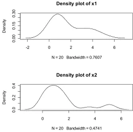
4. Illustrative example

we set LSL1and USL29, the true difference between two process capability indices,

 , is 0.8111. The first random sample (x1) generated is

0.02 0.05 0.32 0.44 0.64 0.64 0.67 0.87 1.05 1.05 1.32 1.33 1.40 2.52 2.80 3.21 3.66 4.11 4.12 5.04.

The second random sample (x2) generated is

0.04 0.14 0.19 0.20 0.23 0.44 0.75 0.81 0.88 1.07 1.07 1.09 1.29 1.50 1.62 1.83 1.91 3.56 5.04 5.15.

In addition, the density plot of generated samples is displayed in Fig. 4.1. Assuming the half logistic distribution for corresponding random variables X1 and X2,three bootstrap

confidence intervals of the difference between two process capability indices with confidence level 95% are constructed, and they are shown in the following table.

Table 5: Bootstrap confidence intervals and widths of the difference between two process capability indices

Methods Confidence intervals Widths

SB ( 0.2441 , 1.2891 ) 1.0450

PB ( 0.3025 , 1.2891 ) 0.9866

BCPB ( 0.2654 , 1.3003 ) 1.0349

As presented in Table 5, the true difference between Cpk1 and Cpk2 ( 0.8111) lies in

the proposed bootstrap confidence intervals. Additionally, the width of CIPB is shorter

than any other confidence intervals by about 5%.

-2 0 2 4 6

0.

00

0.

15

0.

30

Density plot of x1

N = 20 Bandwidth = 0.7607

D

en

si

ty

0 2 4 6

0.

0

0.

2

0.

4

Density plot of x2

N = 20 Bandwidth = 0.4741

D

en

si

5. Conclusions

In this paper, we have proposed bootstrap confidence intervals of the difference between two process capability indices for half logistic distribution. Three bootstrap confidence intervals are considered: the standard bootstrap confidence interval (CISB), the percentile

bootstrap confidence interval (CIPB) and the bias-corrected percentile bootstrap

confidence interval (CIBCPB).The performances of bootstrap confidence intervals are

compared by considering their coverage probabilities and average widths using Monte Carlo experiments. Based on simulation studies, the CIBCPBachieves better coverage

probability than the other bootstrap confidence intervals when  1 1 and 2 2. In

addition, the CIPB performs well with respect to the coverage criterion when  1  1 and

2 2.

  On the other hand, proposed bootstrap confidence intervals are not suitable in terms of coverage probability for other situations ( 1 1 and 2 2).

It would be of interest to propose confidence intervals of the difference between two process capability indices for half logistic distribution when  ₁  ₁ and ₂ ₂, and this is left as a topic for future work.

Acknowledgements

The authors acknowledge the excellent suggestions provided by Professor Dr. R.R.L. Kantam and Professor Dr. David E. Giles. The authors are grateful to Mark Zentz for his careful editing of the manuscript, and to two referees for their constructive comments on an earlier version of this paper.

References

1. Balakrishnan, N. (1985). Order statistics from the half logistic distribution.

Journal of Statistical Computation and Simulation, 20(4): 287-309.

2. Balakrishnan, N. and Aggarwala, R. (1996). Relationships for moments of order statistics from the right-truncated generalized half logistic distribution. Annals of the Institute of Statistical Mathematics, 48(3): 519-534.

3. Balakrishnan, N. and Chan, P.S. (1992). Estimation for the scaled half logistic distribution under Type-II censoring. Computational Statistics & Data Analysis, 13(2): 123-141.

4. Balakrishnan, N. and Saleh, H.M. (2011). Relations for moments of progressively Type-II censored order statistics from half logistic distribution with applications to inference.Computational Statistics & Data Analysis, 55(10): 2775-2792. 5. Balakrishnan, N. and Wong K.H.T. (1994). Best linear unbiased estimation of

7. Efron, B. and Tibshirani, R.J. (1993). An introduction to the bootstrap. Chapman & Hall, New York.

8. Giles, D.E. (2012). Bias reduction for the maximum likelihood estimators of the parameters in the half-logistic distribution. Communications in Statistics-Theory and Methods, 41(2): 212-222.

9. Ihaka, R. and Gentleman, R. (1996). R: A language for data analysis and graphics. Journalof Computational and GraphicalStatistics, 5(3): 299-314.

10. Jang, D.H., Park, J. and Kim, C. (2011). Estimation of the scale parameter of the half-logistic distribution with multiply Type II censored sample. Journal of the

KoreanStatisticalSociety, 40(3): 291-301.

11. Kane, V.E. (1986). Process capability indices. Journal of Quality Technology,

18(1): 41-52.

12. Kang, S.B., Cho, Y.S. and Han, J.T. (2008). Estimation for the half logistic distribution under progressive Type-II censoring. Communications of the Korean

Mathematical Society, 15(6): 815-823.

13. Kantam, R.R.L. and Rosaiah, K. (1998). Half logistic distribution in acceptance sampling based on life tests. IAPQR Transactions: Journal of the Indian

Association for Productivity, Quality & Reliability,23(2): 117-125.

14. Kantam, R.R.L., Rosaiah, K. and Anjaneyula, M.S.R. (2000). Estimation of reliability in multicomponent stress-strength model: half logistic distribution.

IAPQR Transactions: Journal of the Indian Association for Productivity, Quality & Reliability, 25(2): 43-52.

15. Kantam, R.R.L., Rosaiah, K. and Subba Rao, R. (2010). Estimation of process capability index for half logistic distribution. International Transactions in

Mathematical Sciences andComputer,3(1): 61-66.

16. Mbah, A.K. and Tsokos, C.P. (2008). Record values from half logistics and inverse weibull probability distribution functions. Neural, Parallel & Scientific Computations, 16(1): 73-92.

17. Olapade, A.K. and Ojo, M.O. (2002). Characterizations of the Logistic Distribution.Nigerian Journal of Mathematics and Applications, 15(1): 30-36. 18. Peng, C. (2010). Estimating and testing quantile-based process capability indices

for processes with skewed distributions.Journal ofData Science, 8(2): 253-268. 19. Rosaiah, K., Kantam, R.R.L. and Srinivasa, R.B. (2009). Reliability test plan for

half logistic distribution.Calcutta Statistical Association Bulletin, 61: 241-244. 20. Satyaprasad, R. (2007). Half logistic software reliability growth model, Ph.D.

Thesis, Acharya Nagarjuna University, India.

21. Srinivasa, R.B. (2004). Control charts and sampling plans in half logistic model, M. Phil Thesis, Acharya Nagarjuna University, India.

22. Tosasukul, J., Budsaba, K. and Volodin, A. (2009). Dependent bootstrap confidence intervals for a population mean.Thailand Statistician, 7(1): 43-51. 23. Zhang, J. (2010). Conditional confidence intervals of process capability indices