Modeling and Optimization of Wire EDM Process With Grey- Taguchi Technique for Super Alloy Material Incoloy-800

e-ISSN: 2278-067X, p-ISSN: 2278-800X, www.ijerd.com

Volume 10, Issue 10 (October 2014), PP.12-21

Modeling and Optimization of Wire EDM Process With

Grey-Taguchi Technique for Super Alloy Material Incoloy-800

Ashok Kumar Choudhary*1, Prof. K. K. Chhabra2

P.hd Student (Mechanical), Faculty of Engineering, Pacific Academy of Higher

Education and Research University, Udaipur

Professor, Faculty of Engineering, Pacific Academy of Higher Education and

Research University, Udaipur

Abstract:- The main purpose of this research work is to investigate the effect and optimization of cutting parameters : pulse on time (Ton), pulse off time (Toff), spark gap voltage (SGV), peak current (IP) and wire feed rate (WFR) on the control parameters material removal rate, surface roughness, gap current and kerf width in wire electrical discharge machining (WEDM). The experiment is planed as per Taguchi design methodology.The Incoloy 800 is chosen for design of experiment with L27 orthogonal array. A Grey analysis is

used for optimal combination of process parameter for rough and finish cutting. These optimal results are comparing with Grey-Taguchi method and find out the best solutions. A regression model validate with regression-ANOVA results.

Keywords:- Wire Electrical Discharge Machining (WEDM), Grey relation analysis, Regression model

I.

INTRODUCTION

The manufacturing industries have demands of better finish, low tolerance, higher production rate, etc for newer and harder materials like titanium, hardened steel, high strength temperature super alloys, fiber-reinforced composites and ceramics [1]. Due to difficulties occur with conventional machining operation, Electrical discharge machining (EDM) method is the best option to machine hard and nonconductive composites. Wire electrical discharge machining (WEDM) is a unique form of EDM [2]. Wire electrical discharge machining is a nontraditional widely accepted machining process used in tool & die industry, aerospace, surgical, automotive, nuclear industries due to its ability to cut materials very hard materials, which are difficult to cut by conventional machining process. In WEDM there is no contact between tool and work piece [3]. WEDM is able to machine any material irrespective of its hardness, brittleness or toughness with highest accuracy due to its electro-thermal machining process [4]. The dielectric water has a number of functions including insulation, ionization, cooling, and removal of waste metal particles. While the voltage builds up, the water ionizes and behaves as a conductor. After the spark, which develops great heat, the water flushes away the eroded material [5].

II.

EXPERIMENTAL SETUP

2.1 WORK MATERIAL

Figure 1: Sample Specimen

2.2 MACHINE SET UP

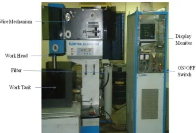
The experiments are carried out on a wire cut EDM machine (ELEKTRA MAXICUT 734) of Electronica Machine Tool Ltd. Installed at MSME Development Institute, Jaipur (Raj.) India, shown in figure 2. In this experiment the upper and lower de-ionized water pressure are 60 litre/min and 40 litre/min respectively. The conductivity of water is set at 50 mho with a temperature of (26±2) °c. The wire tension is set at 800 kgf.

Figure 2: ‘ELEKTRA MAXICUT 734’, Electronica Machine Tool Ltd

2.3 DATA COLLECTION

Figure 3: Mitutoyo Projector Surftest

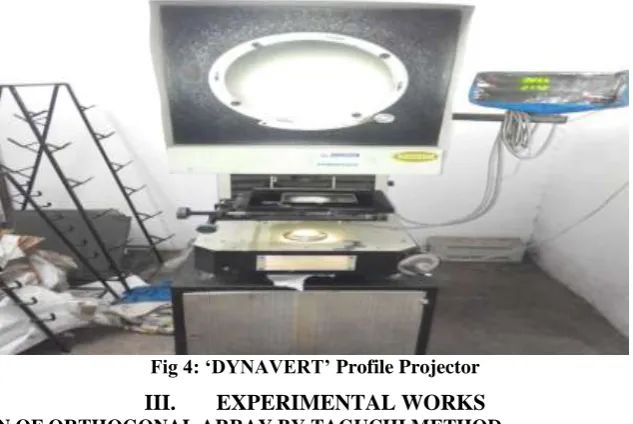
The kerf width of specimen is measured by „DYNAVERT‟ PROFILE PROJECTOR shown in figure 4. The least count of this optical profile projector is 0.005mm

Fig 4: ‘DYNAVERT’ Profile Projector

III.

EXPERIMENTAL WORKS

3.1 SELECTION OF ORTHOGONAL ARRAY BY TAGUCHI METHOD

Control factors along with their levels are listed in Table 1. The Taguchi method is used to create the experimental layout, to analyze the effect of each parameter on the machining characteristics. This method predicts the most favorable selection for WEDM process parameter [6]. The purpose of ANOVA experimentation is to decrease and control the deviation of a process. ANOVA is the algebraic method used to read experimental data to make the essential decisions. [7]

TABLE 1: PROCESS PARAMETER AND THEIR LEVELS

Factors Process parameters Units Levels Selected

Level 1 Level 2 Level 3

A Pulse on time (Ton) µs 3 4 5

B Pulse off time (Toff) µs 2 3 4

3.2 GREY RELATIONAL

3.2.1 Grey Relational Analysis (GRA)

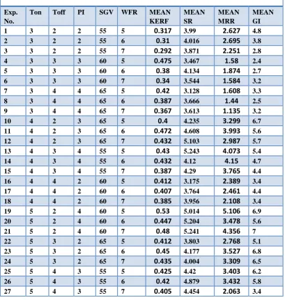
In grey relational study, at first experimental data are normalized ranging from zero to one. After that, based on normalized experimental data, grey relational coefficient is calculated to signify the relationship between the desired and actual experimental data. The overall grey relational grade is determined as a result of averaging the grey relational coefficient related to responses parameter. The overall performance characteristics of response process are controlled by the calculated grey relational grade [9]. The weighting factors (w) are selected as their sum is equal to one. A higher weighting factor for an objective indicates more accurate on it [8].The process parameter and mean response parameter are shown in table 2.

TABLE 2: PROCESS PARAMETER AND MEAN RESPONSE PARAMETER

Exp. No.

Ton Toff PI SGV WFR MEAN

KERF

MEAN SR

MEAN MRR

MEAN GI

1 3 2 2 55 5

0.317

2.627

2 3 2 2 55 6

0.31

2.695

3 3 2 2 55 7

0.292

2.251

4 3 3 3 60 5

0.475

1.58

5 3 3 3 60 6

0.38

1.874

6 3 3 3 60 7

0.34

1.584

7 3 4 4 65 5

0.42

1.608

8 3 4 4 65 6

0.387

1.44

9 3 4 4 65 7

0.367

1.135

10 4 2 3 65 5

0.4

3.299

11 4 2 3 65 6

0.472

3.993

12 4 2 3 65 7

0.432

2.987

13 4 3 4 55 5

0.43

4.073

14 4 3 4 55 6

0.432

4.15

15 4 3 4 55 7

0.387

3.765

16 4 4 2 60 5

0.412

2.389

17 4 4 2 60 6

0.407

2.461

18 4 4 2 60 7

0.385

2.108

19 5 2 4 60 5

0.53

5.106

20 5 2 4 60 6

0.447

3.478

21 5 2 4 60 7

0.48

4.356

22 5 3 2 65 5

0.412

2.768

23 5 3 2 65 6

0.45

3.527

24 5 3 2 65 7

0.435

3.309

25 5 4 3 55 5

0.425

3.403

26 5 4 3 55 6

0.42

3.432

27 5 4 3 55 7

0.405

2.063

A higher grey relational grade results better product quality. On the basis of the grey relational grade, the factor effect is predictable and the optimal level for each process parameter can also be determined [12].The Gray Relationship generating approach is adopted to change the original sequence factor space into measurable space. It generates a comparable sequence with three different comparability types: Larger-the-Better,

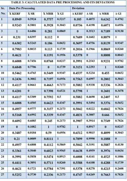
Smaller-TABLE 3: CALCULATED DATA PRE PROCESSING AND ITS DEVIATIONS

Sr.

No.

Data Pre Processing Deviation

X KERF X SR X MRR X GI Δ KERF Δ SR Δ MRR Δ GI

1

_0.8949

_0.3757

_0.105

_0.6242

2

_0.9243

_0.3928

_0.0756

_0.6071

3

₁

_0.281

₀

_0.7189

4

_0.231

_0.112

_0.7689

_0.8879

5

_0.6302

_0.186

_0.3697

_0.8139

6

_0.7983

_0.113

_0.2016

_0.8869

7

_0.4621

_0.1191

_0.5378

_0.8808

8

_0.6008

_0.0768

_0.3991

_0.9231

9

_0.6848

₀

_0.3151

₁

10

0.5462

0.5449

0.4537

0.455

11

0.2436

0.7197

0.7563

0.2802

0.4117

0.4663

0.5882

0.5336

13

0.4201

0.7398

0.5798

0.2601

14

0.4117

0.7592

0.5882

0.2407

15

0.6008

0.6623

0.3991

0.3376

0.4957

0.3157

0.5042

0.6842

17

0.5168

0.3339

0.4831

0.666

18

0.6092

0.245

0.3907

0.7549

19

0

1

1

0

20

0.3487

0.59

0.6512

0.4099

21

0.21

0.8111

0.7899

0.1888

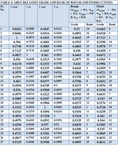
for MRR and relatively higher importance to dimensional accuracy in terms of KW and SR. Grey optimization is conducted for both cutting scenarios. In case of optimization for rough cutting, value of 0.40 is selected as weight for MRR, 0.1 for KW, 0.1 for SR and 0.4 for GI. In case of optimization for finish cutting, value of 0.10 is selected as weight for MRR, 0.4 for KW, 0.4 for SR and 0.1 for GI.

TABLE 4: GREY RELATION GRADE AND RANK OF ROUGH AND FINISH CUTTING Sr.

No

γ KERF γ SR γ MRR γ GI Rough

(w_KERF = 0.1, wSR

= 0.1, w_{MRR = 0.4} & w_GI = 0.4)

Finish

(w_KERF = 0.4, w_SR = 0.4, w_MRR = 0.1 & w_GI = 0.1)

Grade Rank Grade Rank

1

0.8263

0.4447

0.52

0.6465

2

0.8686

0.4516

0.4891

0.6518

3

1

0.4101

0.4643

0.7113

4

_0.394

_0.3602

_0.3925

_0.5298

5

0.5748

0.3805

0.4003

0.5078

6

0.7125

0.3605

0.438

0.6458

7

0.4817

0.362

0.4463

0.6672

8

_0.556

_0.3513

_0.3977

_0.5565

9

_0.6134

_0.3333

_0.414

_0.5906

10

_0.5242

_0.5235

_0.6645

_0.5459

11

0.3979

0.6407

0.5864

0.4521

12

0.4594

0.4837

0.5298

0.4355

13

0.463

0.6577

0.5786

0.4432

14

_0.4594

_0.6749

_0.5675

_0.5076

15

_0.556

_0.5968

_0.5297

_0.5196

16

0.4979

0.4222

0.4703

0.6633

17

0.5085

0.4287

0.4725

0.543

18

0.5613

0.3984

0.4275

0.5276

19

_0.3333

₁

_0.8525

_0.4728

20

0.4343

0.5494

0.5456

0.4258

21

0.3876

0.7258

0.7624

0.461

22

0.4979

0.4592

0.5135

0.544

23

0.4296

0.557

0.6839

0.5203

24

_0.4541

_0.5249

_0.6386

_0.535

25

_0.4722

_0.5382

_0.6043

_0.4969

26

0.4817

0.5425

0.5657

0.4632

27

0.5129

0.3948

0.4095

0.4611

From Table 4, it is shown that machining operations for roughing the best rank is recognized to DOE serial 19 which relates to optimal combination of A3B1C3D2E1. The machining operations for finishing the best rank is recognized to DOE serial 3 which relates to optimal combination of A1B1C1D1E3.

3.1.2 Analysis of grey grade by ANOVA

M ea n of S N ra tio s 5 4 3 -4 -5 -6 -7 4 3

2 2 3 4

65 60 55 -4 -5 -6 -7 7 6 5

Ton Toff SV

PI W FR

Main Effects Plot (data means) for SN ratios

Signal-to-noise: Larger is better

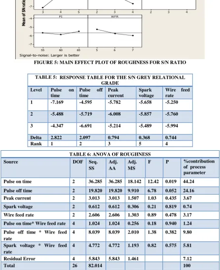
FIGURE 5: MAIN EFFECT PLOT OF ROUGHNESS FOR S/N RATIO

TABLE 6: ANOVA OF ROUGHNESS

Source DOF Seq.

SS

Adj. AA

Adj. MS

F P %contribution

of process parameter

Pulse on time 2 36.285 36.285 18.142 12.42 0.019 44.24

Pulse off time 2 19.820 19.820 9.910 6.78 0.052 24.16

Peak current 2 3.013 3.013 1.507 1.03 0.435 3.67

Spark voltage 2 0.612 0.612 0.306 0.21 0.819 0.74

Wire feed rate 2 2.606 2.606 1.303 0.89 0.478 3.17

Pulse on time* Wire feed rate 4 1.024 1.024 0.256 0.18 0.940 1.24

Pulse off time * Wire feed rate

4 8.039 8.039 2.010 1.38 0.382 9.80

Spark voltage * Wire feed rate

4 4.772 4.772 1.193 0.82 0.575 5.81

Residual Error 4 5.843 5.843 1.461 7.12

Total 26 82.014 100

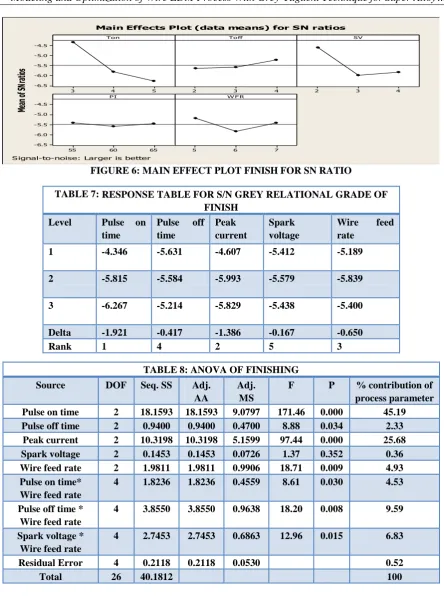
For finishing operation it is found form table and figure that most significant factor is pulse on time and most optimal combination is A1B3C1D1E1.The contribution of pulse on time and peak current are

TABLE 5: RESPONSE TABLE FOR THE S/N GREY RELATIONAL GRADE

Level Pulse on time

Pulse off time

Peak current

Spark voltage

Wire feed rate

1 -7.169 -4.595 -5.782 -5.658 -5.250

2 -5.488 -5.719 -6.008 -5.857 -5.760

3 -4.347 -6.691 -5.214 -5.489 -5.994

Delta 2.822 2.097 0.794 0.368 0.744

Me an of SN ra tio s 5 4 3 -4.5 -5.0 -5.5 -6.0 -6.5 4 3

2 2 3 4

65 60 55 -4.5 -5.0 -5.5 -6.0 -6.5 7 6 5

Ton Toff SV

PI W F R

Main Effects Plot (data means) for SN ratios

Signal-to-noise: Larger is better

FIGURE 6: MAIN EFFECT PLOT FINISH FOR SN RATIO

3.1.3 Conformation test for gray relation

For rough operation the best rank is recognized to DOE serial 19 which relates to combination of A3B1C3D2E1 for a value of 5.106 mm2/min while for the most optimal combination of A3B1C3D3E1 result is 5.338 mm2/min.

For finish operation the best rank is recognized to DOE serial 3 which relates to combination of A1B1C1D1E3 for a value of 3.871µm while for the most optimal combination of A1B3C1D1E1 result is 3.122µm.

TABLE 7: RESPONSE TABLE FOR S/N GREY RELATIONAL GRADE OF FINISH

Level Pulse on

time

Pulse off time

Peak current

Spark voltage

Wire feed rate

1 -4.346 -5.631 -4.607 -5.412 -5.189

2 -5.815 -5.584 -5.993 -5.579 -5.839

3 -6.267 -5.214 -5.829 -5.438 -5.400

Delta -1.921 -0.417 -1.386 -0.167 -0.650

Rank 1 4 2 5 3

TABLE 8: ANOVA OF FINISHING

Source DOF Seq. SS Adj.

AA

Adj. MS

F P % contribution of

process parameter

Pulse on time 2 18.1593 18.1593 9.0797 171.46 0.000 45.19

Pulse off time 2 0.9400 0.9400 0.4700 8.88 0.034 2.33

Peak current 2 10.3198 10.3198 5.1599 97.44 0.000 25.68

Spark voltage 2 0.1453 0.1453 0.0726 1.37 0.352 0.36

Wire feed rate 2 1.9811 1.9811 0.9906 18.71 0.009 4.93

Pulse on time* Wire feed rate

4 1.8236 1.8236 0.4559 8.61 0.030 4.53

Pulse off time * Wire feed rate

4 3.8550 3.8550 0.9638 18.20 0.008 9.59

Spark voltage * Wire feed rate

4 2.7453 2.7453 0.6863 12.96 0.015 6.83

Residual Error 4 0.2118 0.2118 0.0530 0.52

VI.

REGRESSION ANALYSIS

3.2.1 Regression equation

Regression analysis is performed to expose the relationship between process parameter and response parameter [14]. A quadratic regression model is shown by equation no.1

Y = a*A + b*B + c*C + d*D + e*E + f + g*A^2 +h*B^2 + i*C^2 + j*D^2 +k*E^2 + l*A* E + m*B*E + n*C*E ……..(1)

In the above equation a, b, c, d, e, f, g, h, i, j, k, l, m, n etc. are the regression coefficients. These regression coefficients obtained by DataFit software.The value of Y (KW, SR, MRR and GI) is obtained with the help of pulse on time (A), pulse off time (B), peak current (C), spark voltage (D) and wire feed rate (E).

Kerf Width=0.05544*A+0.08361*B+0.09155*C+0.13336*D-0.10363*E-3.79377-0.01233*A^2- 0.00966* B^2-0.01000*C^2-0.00115*D^2-0.00366*E^+0.01383*A*E-0.00475*B*E+0.00150*D*E …… (2)

Surface Roughness = 1.472*A - 1.432*B + 1.402*C - 0.457*D - 0.867*E + 17.783 -0.131*A^2 +0.154*B^2 -

0.189*C^2+0.001*D^2-0.143*E^2+0.001*A*E+0.027*B*E+0.043*D*E …… (3)

Material Removal Rate=5.70533*A+0.54027*B-1.32888*C-0.93427*D+0.89494*E+19.18029 - 0.56744*A^2 -0.13494*B^2+0.26755*C^2+0.005895*D^2-0.20494*E^2-0.05866*A*E-0.05466*B*E+0.02966*D*E . … (4)

Gap Current = 3.766*A - 1.438*B-0.088*C - 2.884*D - 6.355*E+102.399-0.299*A^2+0.116*B^2+0.033*C^2 +0.019*D^2 - 0.000009*E^2 +0.000001*A*E+0.000001*B*E+0.101*D*E ………. …… (5)

3.2.2 Regression equation justification by ANOVA

The deviation of an experiment is finding out by ANOVA experimentation. For MRR, ANOVA results for regression model are shown in table, which shows that the value of P is very close to 0. This value of P indicates that the regression model is fit. Similarly for KW, SR and GI values of P indicates that the regression model is fit.

V.

CONCLUSION

The research work was carried out for analysis surface roughness and material removal rate. The experiments were conducted under various parameter setting. Grey analysis is used for analyze L27 orthogonal array experimental data. Following conclusion is achieved after analysis.

1. The highest grey relation grade for rough cutting was 0.8525 for trial no. 19. The optimal combination of process parameters for rough cutting according to grey analysis was A3B1C3D2E1.

2. The optimal combination of process parameters for rough cutting was A3B1C3D3E1 according to grey -taguchi design method.

3. The highest grey relation grade for finish cutting was 0.7113 for trial no. 3. The optimal combination of process parameters for rough cutting according to grey analysis was A1B1C1D1E3.

4. The optimal combination of process parameters for rough cutting was A1B3C1D1E1 according to grey -taguchi design method.

5. It is shown that the most important parameter for rough and finishing cutting is pulse on time having contribution of 44.24% and 45.19% respectively.

6. The regression equation no. 2, 3, 4 and 5 for KW, SR, MRR and GI respectively are justified by regression-ANOVA results.

TABLE.9 Source DF Sum of

Squares

Mean Square

F Ratio Prob (F)

Regression 13 24.589 1.891 9.349 0.00014

Error 13 2.63 0.202

REFERENCE

[1]. G.Rajyalakshmi and Dr.P.Venkata Ramaiah, “Simulation, Modelling and Optimization of Process parameters of Wire EDM using Taguchi –Grey Relational Analysis”, G. Rajyalakshmi et al. / IJAIR ISSN: 2278-7844

[2]. Kamal Jangra, Sandeep Grover and Aman Aggarwal, “Simultaneous optimization of material removal rate and surface roughness for WEDM of WCCo composite using grey relational analysis along with Taguchi method”, International Journal of Industrial Engineering Computations 2 (2011) 479–490 [3]. D. Sudhakara and G.Prasanthi “ Review of Research Trends: Process Parametric Optimization of Wire

Electrical Discharge Machining (WEDM)” International Journal of Current Engineering and Technology E-ISSN 2277 – 4106, P-ISSN 2347 - 5161

[4]. S.A. Sonawane and M.L. Kulkarni, “Effect of wedm machining parameters on output characteristics”, International Journal of Mechanical and Production Engineering Research and Development (IJMPERD) ISSN 2249-6890 Vol. 3, Issue 2, Jun 2013, 57-62

[5]. Chang-Ho Kim, “ Influence of the Electrical Conductivity of Dielectric Fluid on WEDM Machinability”, Dept. of Mechanical Engineering, Dong-Eui University, Gaya-2 Dong, Pusanjin-Gu, Pusan, 614-714,Korea

[6]. Lokeswara Rao T. and N. Selvaraj, “Optimization of WEDM Process Parameters on Titanium Alloy Using Taguchi Method”, International Journal of Modern Engineering Research (IJMER) Vol. 3, Issue. 4, Jul. - Aug. 2013 pp-2281-2286 ISSN: 2249-6645

[7]. Pujari srinivasa rao, Dr. koona ramji and Prof. Beela satyanarayana “Prediction of Material removal rate for Aluminum BIS-24345 Alloy in wire-cut EDM”, Pujari Srinivasa Rao et al. / International Journal of Engineering Science and Technology Vol. 2 (12), 2010, 7729-7739

[8]. S. S. Mahapatra and Amar Patnaik, “Optimization of wire electrical discharge machining (WEDM) process parameters using Taguchi method”, Published in International Journal of Advanced Manufacturing Technology, 2006

[9]. Saurav Datta and Siba Sankar Mahapatra, “Modeling, simulation and parametric optimization of wire EDM process using response surface methodology coupled with grey-Taguchi technique”, International Journal of Engineering, Science and Technology Vol. 2, No. 5, 2010, pp. 162-183

[10]. M. Durairaj, D. Sudharsun and N. Swamynathan, “Analysis of Process Parameters in Wire EDM with Stainless Steel using Single Objective Taguchi Method and Multi Objective Grey Relational Grade”, The Authors. Published by Elsevier Ltd., Procedia Engineering 64 ( 2013 ) 868 – 877

[11]. S.Balasubramanian and Dr.S. Ganapathy, “Grey Relational Analysis to determine optimum process parameters for Wire Electro Discharge Machining (WEDM)” S.Balasubramanian et al. / International Journal of Engineering Science and Technology (IJEST)

[12]. Muthu Kumar V, Suresh Babu A, Venkatasamy R and Raajenthiren M, “Optimization of the WEDM Parameters on Machining Incoloy800 Super alloy with Multiple Quality Characteristics”, Muthu Kumar.V et al. / International Journal of Engineering Science and Technology Vol. 2(6), 2010, 1538-1547

[13]. Kuo-Wei Lin and Che-Chung Wang, “Optimizing Multiple Quality Characteristics of Wire Electrical Discharge Machining via Taguchi method-based Gray analysis for Magnesium Alloy”, JOURNAL OF C.C.I.T., VOL.39, NO.1, MAY, 2010