Bathymetry Determination from High Resolution Satellite Imagery Using Ensemble Learning Algorithms in Shallow Lakes: Case Study El-Burullus Lake



Abstract—Determination of bathymetric information is key element for near off shore activities and hydrological studies such as coastal engineering applications, sedimentary processes and hydrographic surveying. Remotely sensed imagery has provided a wide coverage, low cost and time-effective solution for bathymetric measurements. In this paper a methodology is introduced using Ensemble Learning (EL) fitting algorithm of Least Squares Boosting (LSB) for bathymetric maps calculation in shallow lakes from high resolution satellite images and water depth measurement samples using Eco-sounder. This methodology considered the cleverest sequential ensemble that assigns higher weights as Boosting for those training sets that are difficult to fit. The LSB ensemble using reflectance of Green and Red bands and their logarithms from Spot-4 satellite image was compared with two conventional methods; the Principal Component Analysis (PCA) and Generalized Linear Model (GLM). The retrieved bathymetric information from the three methods was evaluated using Echo Sounder data. The LSB fitting ensemble resulted in RMSE of 0.15m where the PCA and GLM yielded RMSE of 0.19m and 0.18m respectively over shallow water depths less than 2m. The application of the proposed approach demonstrated better performance and accuracy compared with the conventional methods.

Index Terms—Bathymetry, PCA, GLM, least square boosting.

I. INTRODUCTION

Accurate bathymetric information is so important for costal science applications, shipping navigations and environmental studies of marine areas [1]. Mapping underwater features as rocks, sandy areas, sediments accumulation and coral reefs needs up to date water depths information [2], [3]. Water depths data are essential also for accomplishing sustainable management [4], bathymetric information constitutes a key element hydrological modeling, flooding estimation and degrading or sediments removing [5], [6].

Manuscript received November 25, 2014; revised April 27, 2015. The work was supported by Mission Department, Egyptian Ministry of Higher Education (MoHE), Egypt-Japan University of Science and Technology (E-JUST) and partially supported by JSPS "Core-to-Core Program, B. Asia-Africa Science Platforms".

H. Mohamed and Abdelazim Negm are with the Environmental Engineering Department, School of Energy and Environmental Engineering, Egypt-Japan University of Science and Technology, Alexandria, Egypt (e-mail: [email protected], [email protected]).

M. Zahran is with the Department of Geomatics Engineering, Faculty of Engineering at Shoubra, Benha University, Egypt (e-mail: [email protected]).

O. Saavedra is with the Department of Civil Engineering, Tokyo Institute of Technology, Oookayama, Meguro, Tokyo, Japan. He is also with E-JUST, Egypt (e-mail: [email protected]).

Sonar remains the primary method for obtaining discreet water depth measurements with high accuracy [7]. Single beam sonar on survey vessel can acquire single point depths along sparsely surveying scan lines up to 500 m depths. Multi-beam side scan sonar improves the scanning with wide swath coverage below the vessel scan line resulting better resolution of the resulting sounding [8]. Although these methods gives high accuracy with about 8 cm in 200 m water depths and high spatial resolution of 6 m, they have many limitations. These methods are time consuming, expensive, have low coverage areas and not appropriate for some places as shallow areas with depths less than 3 m [9].

Airborne LIDAR measurements represent another method for accurate water depths detection especially in the last years. LIDAR systems are fast, accurate and appropriate alternative solution for difficult shallow aquatic areas [10]. Some of these LIDAR systems can reach 70 m depths and 20 cm vertical accuracy [11]. Despite of the accuracy of these systems they are limited in coverage compared to satellite images and high costing of operation [12].

Remote Sensing Multi-spectral satellite images are considered the feasible alternative method for bathymetric estimation [9]. These images precede the LIDAR methods in their wide coverage, low costs, high spatial resolution and suitability for shallow areas. Starting in 1978 with areal images over clear shallow waters Lyzenga developed the first empirical methods for estimating bathymetry [13]. In the following years many satellites were lunched with progressive improvements in their spatial and spectral resolutions. Landsat was the first satellite used for bathymetric applications [14], [15] followed by IKONOS [16], and Quick Bird [17], [18]. Recently a new version of high resolution satellite images were used for detecting water depths as instance Spot images [12] and Worldview-2 [19].

Various algorithms were proposed for water depths estimation from optical satellite images depending on the relationship between image pixel values and water depths samples [2]. Lyzenga proposed a methodology depending on the physical Lambert–Beer law of attenuation. A log-linear relationship between corrected image reflectance values and water depths can be used for detecting bathymetric information in certain area. The theory depends on removing the sun-glint and water column effect from images.The resulted differences in reflectance values will be due to changes in water depths [8]-[10].

However this assumption may not be correct for heterogeneous complex areas with different conditions in atmosphere and sun-glint [20]. This method was applied with other satellite images with some improvements in the following years as Landsat [21], Quickbird [22] and [9].

Bathymetry Determination from High Resolution Satellite

Imagery Using Ensemble Learning Algorithms in Shallow

Lakes: Case Study El-Burullus Lake

Hassan Mohamed, Abdelazim Negm, Mohamed Zahran, and Oliver C. Saavedra

Some researchers try to improve this methodology through dividing the area into zones of penetration then calculating the depths in these zones using Hierarchical Markov chain algorithms [23] or splitting the water column into attenuation levels according to turbidity using stratified genetic algorithm [24].

Stumpf [16] proposed another approach using band ratios. Their theory assumes that the effects of different heterogeneous water areas will be the same for two bands and so the ratio between their reflectance values can be used to estimate water depths. Although this theory needs less parameters and less affected with bottom type it does not have sound physical foundation and needs pre coefficients selected with trial and error by the user. Su [2] try to calibrate the parameters for the non-linear inversion model proposed by Stumpf [16] automatically using the Levenberg-Marquardt optimization algorithm.

Martin [25] and Noela [12] used the principal component analysis (PCA) for detecting water depths from satellite images. The principal component of the log transformed reflectance was linearly correlated with water depths samples.

The methodology proposed in this research uses Least Squares Boosting fitting ensemble for estimating water depths in shallow waters. The influencing bands for bathymetry after removing atmosphere and sun glint corrections and their logarithms are used as input data in the ensemble. The proposed approach reduces the water depth measurement requirements, saves time, costs and difficulties of field surveying. The methodology was applied using SPOT-4 imagery of EL-Burullus Lake in Egypt and compared with two other conventional methods. Achieved results were evaluated using Echo-Sounder bathymetric data for the same area.

II. METHODOLOGY

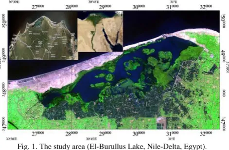
A. Study Area and Available Data

Fig. 1. The study area (El-Burullus Lake, Nile-Delta, Egypt).

A pan-sharped SPOT-4 HRG-2 satellite image with four

multispectral bands is used for detecting bathymetry for the study area. The four bands are green (0.5–0.59 µm), red (0.61–0.68 µm), near-infrared (0.78–0.89 µm) and short-wave infrared (1.58–1.75 µm). The image has 10 m spatial resolution and was acquired on July 1st, 2012 in Fig. 2.

Fig. 2. The SPOT: 4 satellite image of the study area (July 1st_{, 2012).}

In-situ depth measurements of bathymetry were acquired by Echo-Sounder instrument in Fig. 3.

Fig. 3. In-situ depth bathymetry points from Echo-Sounder.

B. Methodology

The following subsections describe the methodology used in this research.

1) Imagery data pre-processing

For detecting bathymetric information from satellite images the radiometric corrected pixel values are firstly converted to spectral reflectance values [28] for all image bands. The required data for this conversion regarding the sensor characteristics in exposure time and the effective band widths for each band are available in the image metadata file. Second, two essential successive steps corrections are applied to the reflectance image; atmospheric correction and Sun-glint correction [9]. The sequence of applying these two corrections is arbitrary. Some researchers start with atmospheric correction followed by sun-glint correction while others reverse this procedure [29]. The following steps summarize the imagery data pre-processing:

Computing theradiance values from image pixel digital numbers using the gain and bias information of sensor bands as follows [29]:

L = DN (Gain) + Bias (1) where:

L = Radiance values for each band

DN = digital numbers recorded by the sensor Gain = the gradient of the calibration

Bias = the spectral radiance of the sensor for a DN of zero. Both gain and bias values were available in the image metadata file.

Calculating the spectral top of atmosphere reflectance of each pixel value using the radiances computed in Eq.2 [30]:

where:

𝝆AS = the top of atmosphere reflectance

d2 = the square value of Earth-sun distance correction in atmospheric units

Esun = exoatmospheric spectral solar constant for each band θz = solar zenith angle

Applying the atmospheric correction to the spectral reflectance image. According to many researchers the preferred method for bathymetry detection is dark pixel subtraction method [17]. The corrected pixel value can be calculated as follows [9]:

Rac = Ri – Rdp (3)

where:

Rac = corrected pixel reflectance value Ri = initial pixel reflectance value Rdp = the dark pixel value.

The dark pixel value is so important for depths determination process and influence the accuracy of depth estimation values [16].

Applying the Sun Glint correction to the image resulted from atmospheric correction process. The sun glint correction can be performed by exploiting the advantage of Near-infrared band which does not contain any bottom reflected signals [2]. Thus the other image bands which contain sun glint areas could be related with the Near-infrared band in linear regression relationship [12]-[32]. The de-glinted pixel value can be easily determined as follows:

Ri' = Ri × bi (RNIR - MinNIR) (4)

where:

Ri' = de-glinted pixel reflectance value Ri= initial pixel reflectance value bi = regression line slope

RNIR = corresponding pixel value in NIR band MinNIR = min NIR value existing in the sample.

Choosing of pixel samples has varying dark, deep and has glint values from the imagery water region influencing the accuracy of results [33].

2) Methods

a) PCA correlation approach

PCA or Multi-band Approach can be used for bathymetry detection through correlating in-situ depth measured values

and reflectance of bands with their logarithms. Therefore, it can use multi-band images for getting more accurate water depths [1]. Image bands are transformed through this approach to new uncorrelated bands known as components ordered by the amount of image variation they can elucidate [34]. The first component resulted from PCA can be correlated to water depths regarding the other environmental factors which have less influence on variation [35].

b) GLM correlation approach

The Generalized Linear Model represents least-squares fit of the link of the response to the data. GLM links a linear combination of non-random explanatory variables X as example image bands to dependent random variable Y as instance the water depths values [36]. The mean of the nonlinear observed variable can be fitted to a linear predictor of the explanatory variables a link function using a link function of g [µY] as follow [12]:

g [µY] = βo+

𝛽𝑖 𝑋𝑖

𝛽𝑖𝑗 𝑋𝑖

𝑋𝑗

where: βo, βi and βij are coefficients and Xi, Xj are variables combinations.

c) Least squares boosting fitting ensemble for bathymetry estimation

Ensemble is a collection of predictors combined with weighted average of vote in order to provide overall prediction that take its guidance from the collection itself [37]. Boosting is considered as one of the most powerful learning ensemble algorithms proposed in the last three decades. It was originally designed for classification but it was found that it can be extended to regression problems [38]. Its an ensemble technique in which learners are learn sequentially with early learners fitting simple models of data and then the data are analyzed from errors. Those errors identifies problems of particular instances of data that are difficult or hard to fit. Later models focus primarily on those instances to try predicting them right. In the end all models are given weights and the set is combined into some overall predictors. Thus boosting is a method of converting a sequence of week learners into very complex predictors or a way of increasing complexity of primary model. Initial learners often are very simple and then the weighted combination can develop more complex learners in Fig. 4. The basic concept of boosting is developing multiple models in sequence by assigning higher weights as boosting for those training cases or learners that are difficult to be fitted in regression problems or classified in classification problems [39].

The predictive learning problem usually consisting of a random output variable (Y) that may be called a response and a set of random input variables (X = X1 … Xn) may be called explanatory. A training sample (Yi, Xi)N of known (Y, X) values is used for obtaining an estimation or approximation F(X), of the function F*(X) for correlating or mapping x to y, in order to minimize the expected value of some specified loss function L(Y, F(X)) over the joint distribution of all (Y, X) values [40]:

F* = arg min EY, xL (Y, F(X)) = arg min EX [EY (L(Y, F(X))) | X] (5) For Y є R (Regression problems) loss functions L(Y, F) International Journal of Environmental Science and Development, Vol. 7, No. 4, April 2016

𝝆AS = 𝜋 𝑑2𝐿

Esun 𝑐𝑜𝑠𝑧 (2)

Least-Squares algorithm can be used to minimize any differentiable loss L(y, F) in conjunction with forward

stage-wise additive modeling for fitting the generic function

h (X, a) to the pseudo-responses (F = -gm(Xi)) for i=1 … N. In Least-squares regression the loss function is L(Y, F) = (Y-F)2/2 and the pseudo-response is Ῡi = Yi - Fm-1 (Xi). The following steps illustrate Least-Squares Boosting algorithm [42]:

Fo(X) = Ῡ

For m = 1 to M do: Ῡi = Yi- Fm-1 (Xi), i = 1, N

(ρm, am)= arg mina, p 𝑁𝑖=1[Ῡi − ρℎ(Xi; 𝐚)]2

Fm(X) = Fm-1 (X) + ρmh (X; am) end For

end Algorithm

As a result, gradient boosting on squared-error loss produces the normal stage-wise approach of iteratively fitting the current residuals [43].

Fig. 4. Boosting example a sequence of learned models and their error residuals where (a) represents single decision model, (b) represents its error residuals and (i) represents sum of five decision models [37].

III. RESULTS AND DISCUSSION

The SPOT-4 multispectral image of the study area was pre-processed for water depths estimation employing two successive steps.

First, image pixel values were converted to radiances then to reflectance utilizing image metadata file values. Second, the atmospheric correction and sun-glint removal were applied to image reflectance values. These two steps were performed in Envi software environment.

The three approaches PCA, GLM and Least Squares Boosting ensemble were applied to the pre-processed Spot-4 multispectral image. A prototype software is developed in Matlab environment to implement the used approaches. The details can be listed as follows:

with R2 = 0.479 Principle Component fitted continuous model showed in Fig. 5.

Fig. 5. 3rd order polynomial continuous fitted model using PC1.

2) The Generalized Linear Model represents a least-squaresfit of the link of the response to the data. As a result a linear combination of green and red corrected bands (GB, RB) and their logarithms (LG, LR) were linked to the water depths values by GLM in the form: regularly include squared-error (Y-F)2and absolute error | Y

-F|. F(x) can be restricted to be a member of a parameterized class of functions F (X; P). As example of this process the additive expansions [40]:

F(X; (βm,am)M) = 𝑀𝑚 =1

𝛽𝑚

h(X,a) is generic function a simple parameterized function of the input variables X.

amthe parameters which characterized the generic function. βm the set of parameters whose joint values identify regression functions. In Boosting case each function of h(X, a) is a regression tree with parameters amas splitting variables. This expansion is included in many approximation methods as Neural Network, Support Vector Machine and Wavelets…etc. [41].

1) The Principle Component Algorithm was applied to the green and red corrected bands and their logarithms. Afterwards, the first principle component (PC1) was correlated with 3rdorder polynomial to the water depths values in the form:

Z = 1050.8 + 17562 GB – 12903 RB + 5.7432 LG – 14.6 Lr –7211.8 GBRB – 5863.1 GB LG +9543.7 RB Lr+ 8188.8 GB

Lr–7139.7 RB LG–72.058 LG Lr (8) with R2 = 0.527 GLM fitted continuous model showed in Fig. 6.

Fig. 6. GLM continuous fitted model. Depths are represented as points and continuous line represents the fitted continuous model.

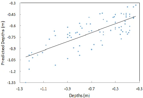
3) Least Squares Boosting ensemble uses the green and red bands and their logarithms as input values and Water depths as output values. The data set was divided to independent training and testing sets for evaluating the performance quality of ensemble with 75% of data set for learning and 25% for testing. After many trials, the appropriate number of regression trees was determined based on the least RMSE and best R2 value and was found to be 50 trees.

The best performance was achieved using 50 trees and resulted in R2 = 0.618 in Fig. 7.

Fig. 7. Least squares boosting continuous fitted model.

Finally the RMSE of all methods was computed using the differences among each model values and actual depths. The results listed in Table I.

compared to conventional methods. Also reducing the in-situ depths required for water depths estimation.

IV. CONCLUSION

In this research, a methodology was developed using bands corrected from atmospheric and sun-glint systematic errors which influencing bathymetry and their logarithms as an input values in Least Squares Boosting ensemble. To validate the precedency of the proposed methodology to other conventional approaches a comparison was applied with two approaches using SPOT-4 satellite image for EL-Burullus (shallow Lake) with depths less than 2 m. All approaches were tested by data collected using Echo-Sounder for measuring water depths. The first approach; PCA 3rd order polynomial correlation algorithm using the first principle component gave RMSE of 0.19 m. The GLM with reflectance of Green, Red bands and their logarithms yielded RMSE of 0.18 m. The proposed methodology using Least Squares Boosting ensemble with reflectance of Green, Red bands and their logarithms as input values with less observed field measurements resulted in RMSE of 0.15 m which outperformed other conventional methods. It can be concluded that Least Squares Boosting ensemble gives more accurate results than conventional methods for bathymetric determination applications.

ACKNOWLEDGMENT

Hassan Mohamed would like to thank Egyptian Ministry of Higher Education (MoHE) for granting him the PhD scholarships. Thanks are also due to Egypt-Japan University of Science and Technology (E-JUST) and JICA for their support and for offering the tools needed for this research. Corps of Engineers are appreciated for their great and continuous technical support. This work was partially supported by JSPS "Core-to-Core Program, B.Asia-Africa Science Platforms".

REFERENCES

[1] O. Ceyhun and A. Yalçın, “Remote sensing of water depths in shallow waters via artificial neural networks,” Estuary. Coast. Shelf Sci., vol. 89, pp. 89–96, 2010.

[2] H. Su, H. Liu, and W. Heyman, “Automated derivation for bathymetric information for multispectral satellite imagery using a non-linear inversion model,” Marine Geodesy, vol. 31, pp. 281-298, 2008. [3] D. Jupp, “Background and extension to depth of penetration (DOP)

mapping in shallow coastal waters,” presented at the Symposium of Remote Sensing of the Coastal Zone, Gold Coast, Queensland, IV.2.1-IV.2.19, September 1988.

[4] J. Gao, “Bathymetric mapping by means of remote sensing: Methods, accuracy and limitations,” Progress in Physical Geography, vol. 33, no. 1, pp. 103–116, 2009.

[5] J. Brock, C. Wright, T. Clayton, and A. Nayegandhi, “LIDAR optical rugosity of coral reefs in Biscayne National Park,” Coral Reefs, Florida, vol. 23, pp. 48–59, 2004.

[6] C. Finkl, L. Benedet, and J. Andrews, “Interpretation of seabed geomorphology based on spatial analysis of high-density airborne laser bathymetry,” Journal of Coastal Research, vol. 21, pp. 501–514, 2005. [7] L. Leu and H. Chang, “Remotely sensing in detecting the water depths and bed load of shallow waters and their changes,” Ocean Engineering, vol. 32, pp. 1174-1198, 2005.

[8] M. Loomis, “Depth derivation from the worldview-2 satellite using hyperspectral imagery,” M.S. thesis, from Naval postgraduate school Monterey, California, March 2009.

[9] G. Doxania, M. Papadopouloua, P. Lafazania, C. Pikridasb, and M. Tsakiri-Strati, “Shallow-water bathymetry over variable bottom types using multispectral Worldview-2 image,” International Archives of the International Journal of Environmental Science and Development, Vol. 7, No. 4, April 2016

TABLE I: THE ROOTMEAN SQUARE ERROR OF DERIVED DEPTHS BY THE

THREE METHODS

Methodology PCA 3

rd

Polynomial

GLM Least Square Boosting RMSE 0.19 m 0.18 m 0.15 m

Photogrammetry, Remote Sensing and Spatial Information Sciences, vol. XXXIX-B8, Melbourne, Australia, 2012.

[11] G. Chust, M. Grande, I. Galparsoro, A. Uriarte, and A. Borja, “Capabilities of the bathymetric hawk eye LIDAR for coastal habitat mapping: A case study within a basque estuary,” Coastal and Shelf

Science, Estuarine, vol. 89, no. 3, pp. 200–213, 2010.

[12] N. Sánchez-Carneroab, J. Ojeda-Zujarb, D. Rodríguez-Pérezc, and J. Marquez-Perez, “Assessment of different models for bathymetry calculation using SPOT multispectral images in a high-turbidity area: The mouth of the Guadiana Estuary,” International Journal of Remote Sensing, vol. 35, no. 2, pp. 493–514, 2014.

[13] D. Lyzenga, “Passive remote sensing techniques for mapping water depth and bottom features,” Applied Optics, vol. 17, pp. 379-383, 1978. [14] D. Lyzenga, “Remote sensing of bottom reflectance and other attenuation parameters in shallow water using aircraft and Landsat data,” Int. J. of Remote Sensing, vol. 2, no. 1, pp. 71-82, 1981. [15] D. Lyzenga, “Shallow-water bathymetry using combined Lidar and

passive multispectral scanner data,” International Journal of Remote Sensing, vol. 6, no. 1, pp. 115-125, 1985.

[16] R. Stumpf, K. Holderied, and M. Sinclair, “Determination of water depth with high-resolution satellite imagery over variable bottom types,” Limnol. Oceanogr, vol. 48, pp. 547-556, 2003.

[17] D. Mishra, S. Narumalani, D. Rundquist, and M. Lawson, “Benthic habitat mapping in tropical marine environments using quick bird multispectral data,” Photogrammetric Engineering & Remote Sensing, vol. 72, pp. 1037–1048, 2006.

[18] C. Conger, E. Hochberg, C. Fletcher, and M.Atkinson, “Decorrelating remote sensing color bands from bathymetry in optically shallow waters,” IEEE Transactions on Geoscience and Remote Sensing, vol. 44, no. 6, pp.1655–1660, 2006.

[19] S. Liew, C. Chang, and L. Kwoh, “Sensitivity analysis in the retrieval of turbid coastal water bathymetry using worldview-2 satellite data,” ISPRS Congress, vol. XXXIX-B7, Melbourne, Australia, 2012. [20] W. Philpot, “Bathymetric mapping with passive multispectral imagery,”

Applied Optics, vol. 28, pp. 1569–1578, 1989.

[21] M. Liceaga-Correa et al., “Assessment of coral reef bathymetric mapping using visible landsat thematic mapper data,” International

Journal of Remote Sensing, vol. 23, no. 1, pp. 3–14, 2002.

[22] M. Lyons, S. Phinn, and C. Roelfsema, “Integrating quickbird multi-spectral satellite and field data: Mapping bathymetry, seagrass cover, seagrass species and change in moreton bay,” Australia in

2004-2007. Remote Sens., vol. 3, pp. 42-64, 2011.

[23] J. Provost, C. Collet, P. Rostaing, P. Pérez, and P. Bouthemy, “Hierarchical markovian segmentation of multispectral images for the reconstruction of water depth maps,” Computer Vision and Image

Understanding, vol. 93, no. 2, pp. 155–174, 2004.

[24] M. Gianinetto and G. Lechi, “Söz ma dna algorithm for the batimetric mapping in the lagoon of venice using quickbird multispectral data,”

ISPRS, vol. XXXV, pp. 94–99, Istanbul, 2004.

[25] K. Martin, “Explorations in geographic information systems technology,” Applications in Coastal Zone Research and Management,

Clark Labs for Cartographic Technology and Analysis, Worcester,

Massachusetts and United Nations Institute for Training and Research (UNITAR), vol. 3, Geneva, Switzerland, 1993.

[26] A. El-Adawy, A. Negm, M. Elzeir, O. Saavedra, I. El-Shinnawy, and K. Nadaoka, “Modeling the hydrodynamics and salinity of El-Burullus Lake (Nile Delta, Northern Egypt),” Journal of Clean Energy

Technologies, vol. 1, no. 2, March 2013.

[27] E. Ali, “Impact of drain water on water quality and eutrophication status of Lake Burullus, Egypt, a southern Mediterranean lagoon,”

African Journal of Aquatic Science, vol. 36, no. 3, pp. 267–277, 2011.

[28] T. Updike and C. Comp. (2010). Radiometric use of worldview-2 imagery. Technical Note. [Online]. Available: https://www.digitalglobe.com/sites/default/files/Radiometric_Use_of_ WorldView-2_Imagery%20 (1).pdf

[29] S. Kay, J. Hedley, and S. Lavender, “Sun glint correction of high and low spatial resolution images of aquatic scenes: A review of methods for visible and near-infrared band wavelengths,” Remote Sens., vol. 1, pp. 697-730, 2009.

[30] S. Goslee, “Analyzing remote sensing data in R: The landsat package,”

Journal of Statistical Software, published by the American Statistical Association, vol. 43, no. 4, 2011.

[31] Landsat-7. (2011). Landsat Science Data Users Handbook. [Online]. Available:

http://landsathandbook.gsfc.nasa.gov/data_prod/prog_sect11_3.html

[32] J. Hedley, A. Harborne, and P. Mumby, “Simple and robust removal of sun glint for mapping shallow-water benthos,” International Journal of

Remote Sensing, vol. 26, no. 10, pp. 2107–2112, May 2005.

[33] A. Edwards. (2010). Les. 5: Removing sun glint from compact airborne spectrographic imager (CASI) imagery. [Online]. Available: http://remotesensing.utoledo.edu/pdfs/less2/Lesson05NQ.pdf [34] A. Hladnik, “Image compression and face recognition: Two image

processing applications of principal component analysis,”

International Circular of Graphic Education and Research, vol. 6, 2013.

[35] M. Gholamalifard, T. Kutser, A. Esmaili-Sari, A. Abkar, and B. Naimi, “Remotely sensed empirical modeling of bathymetry in the southeastern caspian sea,” Remote Sens., vol. 5, pp. 2746-2762, 2013. [36] M. Marlene, “Generalized linear models,” Handbooks of

Computational Statistics, pp. 681-709, Springer-Verlag, Berlin,

Heidelberg, 2011.

[37] A. Ihler, “Ensembles of learners,” presented at Machine Learning and Data Mining, Bern ICS Information and Computer Science, University of California, 2012.

[38] T. Hastie, R. Tibshirani, and J. Friedman, “The elements of statistical learning data mining, inference, and prediction,” Springer Series in Statistics, 2nd ed., Stanford, California, 2008.

[39] J. Quinlan. (2006). Bagging, Boosting and C4.5. [Online]. Available: http://www.cs.utah.edu/~piyush/teaching/Quinlan.AAAI96.pdf [40] J. Freidman, “Greedy function approximation: A gradient boosting

machine,” The Annals of Statistics, vol. 29, no. 5, pp. 1189-1232, Institute of Mathematical Statistics, October, 2001.

[41] D. Rumelhart, G. Hinton, and R. Williams, “Learning internal representations by error propagation,” Parallel Distributed Processing,

Cambridge, MA: MIT Press, vol. 1, pp. 318-362, 1986.

[42] P. Casale, O. Pujol, and P. Radeva, “Embedding random projections in regularized gradient boosting machines,” presented at Ensembles in Machine Learning Applications, pp. 201-216, Heidelberg, Berlin: Springer-Verlag, 2011.

[43] P. Bühlmann, “Boosting for high-dimensional linear models,” Institute of Mathematical Statistics, the Annals of Statistics, vol. 34, no. 2, pp. 559–583, 2006.

Hassan Mohamed was born in 1984 at Cairo, Egypt.

He has got his bachelor of science degree in civil engineering (geomantics oriented), Faculty of Engineering at Shoubra, Benha University, Egypt in 2006. Hassan’s master degree of science was in remote sensing and GIS from Geomantics Dept., Faculty of Engineering at Shoubra, Benha University, Egypt in 2012. Now, he is a PhD student at E-JUST. He worked as a demonstrator at the Geomantics Engineering Department, Faculty of Engineering at Shoubra, Benha University, Egypt from 2007 to 2012. From 2012 till now, he has been an assistant lecturer at the Geomantics Engineering Department, Faculty of Engineering at Shoubra, Benha University, Egypt.

Abdelazim Negm was born in Sharkia, Egypt. His

background is civil engineering because he was graduated from Irrigation and Environmental Engineering Dept. in 1985. Prof. Negm has got his M.Sc. degree from Ain Shams University in 1990 in hydrology of the Nile basin. He got the PhD degree in 1992 in hydraulics. Currently, he is a professor of water resources in Egypt-Japan University for Science and Technology (E-JUST) since Oct. 2012 and the chairman of the Environmental Engineering Dept. at E-JUST since Feb. 17, 2013. He worked as a demonstrator in Faculty of Engineering, Zagazig University in 1986 and continued till he occupied the position of vice dean for Academic and Student Affair. He was promoted as a professor of hydraulics. His research areas are wide to include hydraulic, hydrology and water resources. He published about 200 papers in national and international journals and conferences. He is listed in (a) Marquis Who is Who?, (b) IBC's 2000 Outstanding Intellectuals of the 21st Century , and (c) ABI directory for his achievement in the field of Hydraulics and Water Resources. He participated in more than 55 conferences. He has awarded the prizes of best papers three times. He participates in the two EU funded international projects. For his detailed information one can visit his websites www.amneg.name.eg and www.amnegm.com.

[10] G. Guenther, A. Cunningham, P. LaRocque, and D. Reid, “Meeting the accuracy challenge in airborne lidar bathymetry,” in Proc. 20th EARSeL Symposium, Workshop on LIDAR Remote Sensing of Land

and Sea, European Association of Remote Sensing Laboratories, Paris,

Mohamed Zahran is a professor in civil engineering (surveying and photogrammetry oriented). He was graduated from the Department of Geomantics Engineering Faculty of Engineering at Shoubra, Benha University in 1984. Prof. Zahran has got his M.Sc. degree from the Department of Civil Engineering, Faculty of Engineering, Cairo University in 1989. He got the PhD degree from the Department of Civil and Environmental Engineering and Geodetic Science, The Ohio State University in 1997. Currently, he is a professor of surveying and photogrammetry in Faculty of Engineering at Shoubra, Benha University since 2008 and a chairman of the Department of Geomatics Engineering Faculty of Engineering at Shoubra, Benha University since 2013. His research areas are wide to include digital photogrammetry, digital image analysis, remote sensing for mapping and close-range photogrammetry. He published many papers in national and international journals and conferences.

、

Oliver C. Saavedra is a PhD in civil engineering (applied hydrology oriented). He is an associate professor at Tokyo Institute of Technology and for adjunct professor to E-JUST since January 2010 to present. He has four years teaching experience in advanced hydrology, GIS, water resources management lectures at graduate school. His major research interests are in development of decision supporting tools for water resources management including optimal dam operation, flood control. He has about three years’ experience as a researcher (hydrology and WRM) and two years’ experience as a consultant engineer (water supply, sanitation, and infrastructure) and two years’ experience as a hydraulic engineer (water distribution systems). His project coordinator is “Integrated water resources and environmental management for Asian and African mega-delta under climate change effects”.