Enhancement the Heat Transfer Coefficient for Three-Phase Flow (water, gasoil, air) Through a Rectangular Channel by Triangular Ribs

(1)

IJENS © October 2017 IJENS

-IJMME -9 8 9 8 -705 4 17

Enhancement the Heat Transfer Coefficient for

Three-Phase Flow (water, gasoil, air) Through a

by Triangular Ribs

Rectangular Channel

2

wared

-and Hassanein J. Al

1

Turaihi

-iyadh S. Al

R

Iraq Mechanical Engineering, University of Babylon, Hilla, Department of

,2 1

[email protected] mail:

-E 2 [email protected] :

mail -E 1

Abstract-- Heat transfer inside vertical rectangular channel for three-phase flow (water-gasoil-air) over triangular ribs have been investigated experimentally and numerically. Four values of water superficial velocity, three values of gasoil superficial velocity and three values of air superficial velocity with three values of heat flux have been investigated. Ansys fluent 15.0 and standard k- ε mixture model have been done for numerical study. Also, determining dimensionless roughness parameter such as rib height to hydraulic diameter ratio (e/Dh) and rib pitch to rib height ratio (P/e) have been

done numerically. Conservation equation of continuity, momentum and energy was solved for the same variables that used experimentally. The local heat transfer coefficient results were found experimentally and compared with the computational results and they were in good agreement with a deviation of about (2.092 % - 14.657 %) for case effect water superficial velocity, about (2.58% - 17.545%) for case effect gasoil superficial velocity and about (1.588 % -16.594 %) for case effect air superficial velocity.

Index Term-- heat transfer; three-phase flow; ribs; vertical rectangular channel; dimensionless roughness parameter.

INTRODUCTION

To improve heat transfer in heat transfer devices, several techniques have been employed for more compact heat transfer system and cost/energy saving. One of the most effective methods of enhancing the heat transfer rate in a smooth channel is the use ribs which are often used to enhance forced convective heat transfer. There are many researches in the field ribs with single phase flow, two-phase flow and a few of it or limited with three-phase flow. Jaurker A. R. et al. 2006, investigated experimentally heat transfer performance in a rectangular solar air heater duct by using rib-grooved and rib without groove. They use comparison with a smooth plate for Re and roughness parameters such as relative roughness pitch (p/e) and relative roughness height (e/Dh) for given values of groove position. The results showed for Nu is higher than the smooth case. Ansari and Arzandi 2012,

experimentally studied the effect of height ribs on the flow pattern by taken three different values for heights rectangular ribs with three different positions, two phase flow air side at top wall, water side at the bottom wall and both of them. Results show the transition boundary line between the stratified and the plug flow patterns occurred at higher liquid velocities and the transition line between the slug and the plug flow pattern occurred at lower gas velocities. Asano et al. 2004, experimentally studied the adiabatic two-phase flow (water-air) and R141b boiling two-phase flow in heat exchangers with a single channel located vertically. They divided flow patterns into two

groups, depended on the gas flow rate, firstly when the gas flow rate was little air flowed in water intermittently. Secondly, when the gas flow rate was a higher, air and water phases flowed continuously. AL-Turaihi 2016, studied experimentally the effect of the discharge of gas and liquid, the particle amount on pressure distribution for liquid-gas-solid three- phase flow in horizontal pipe. Results show increase pressure magnitude at increasing loading ratio, water discharge and air discharge.Lawrence and Panagiota 2014, studied liquid–liquid flows (oil-water) for stratified flow. Using conductance probes, average interface heights were obtained at the pipe center and close to the pipe wall, which revealed a concave interface shape in all cases studied. In addition, from the time series of the probe signal at the pipe center, the average wave amplitude was calculated to be 0.0005 m and was used as an equivalent roughness in the interfacial shear stress model. Weisman et al. 1994, experimentally investigated the patterns and pressure drop of two-phase flow in a horizontal circular pipe with helical wire ribs. the ribs of a circular cross-section were used with different values of heights and different helical twist ratios. Results showed, if the fluid velocity at the entrance of the pipe exceeded the minimum value that depended on experience, so the flow in the pipe be a swirling annular flow at all qualities, and this would improve the heat transfer rate. Yuyuan et al. 1994,

experimentally investigated the influences of nominal gap scales for boiling two-phase flow on the critical heat flux and heat transfer coefficients through a lunate channel. Results show when the scale of nominal gap was less than (2 mm), the heat transfer coefficient increased significantly. Depending on the results, the heat transfer coefficient being improved by nine times of that for bare pipes when the scale of nominal gap about (1 mm).

1.Experimental Apparatus and Procedure:

1.1.Experimental Apparatus

(2)

-IJMME -9 8 9 8 -705 4 17

wool to prevent thermal losses. The experimental equipment’s include the following:

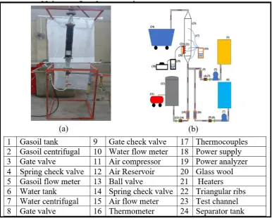
1. Three tanks to store the water, gasoil and air, three centrifugal pumps and three flow meters to measure the flow rate of water, gasoil and air with percentage errors for water flow meter is about (0.5% - 8.5%), for gasoil flow meter is about (0.8% - 6.5%).

2. Air compressor to compressed air to the air tank and then supply the rig.

3. Thermometer to record the temperature reading at different positions of the test channel with percentage error about (0 %-1.61%) with five thermocouples (T type) one on the surface rib and others distributed on the test channel.

4. Valves to control flow discharge and check valves to prevent back flow.

5. Power supply and digital power analyzer.

Fig. 1. (a) Experimental rig (b) Schematic of experimental setup

Fig. 2. Triangle ribs

(3)

-IJMME -9 8 9 8 -705 4 17

1.2. Experimental Procedure.

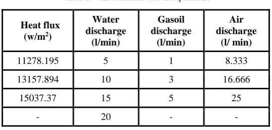
In experimental work one hundred and eight test carried out by taken different values of water, gasoil and air superficial velocities and different values of heat flux as shown in table (1), for the first test is:

1- Turn on the water centrifugal pump at the initial value of (5 l/min).

3- Supply the electrical power to the heaters at the first value (120 watt) which is constant for all thirty-six tests.

4- Wait few minutes (5-10 min) until the rib reach to the desired temperature (46 ºc) by observing the temperature variations in different locations along the test channel.

5-Turn on the gasoil centrifugal pump at the initial value of (1 l/min) and then turn on air compressor at the initial value of (8.333 l/min).

6- Recording the temperature by sensors which are located at five points four of them along the test channel and one for the rib surface as well as, with recording video to observe the flow behavior.

7- Change the second value of air volume flow rate with still water and gasoil values constant and repeat the above steps until to finish all the air volume flow rate values.

8- Change the second value of gasoil volume flow rate with still water value is constant, repeat the above steps until to finish all the gasoil volume flow rate values.

9- Repeat all above steps with a new water volume flow rate value until to finish all the water volume flow rate.

Table I

Values of work conditions used in experiments

2. Data Reduction

2.1 Superficial Velocity

Superficial velocities were found for water, gasoil and air from Eq. (1) where the fluid flow rate was measured directly from the flow meter (Asano et al. 2004; Ansari and Arzandi. 2012),

U



Q

A

... (1)

Also, to calculate the Reynolds Number need to make assumptions to calculate the working fluid properties. Where the working fluids in a present study are water, gasoil and air which have different properties. For example, the water and gasoil density are relatively a thousand times greater than air density so water-gasoil-air three-phase flow can be simplified into gas-liquid two-phase flow but still complex. Fluid properties Such as density and viscosity depend on continuous phase and fraction dispersed phase as shown below (Hanafizadeh P. et al. 2017). In this study water is continuous phase and dispersed phase is gasoil and air.

... (2)

ρm = ρc (1+α) …… (3) ……. (4)

a

+ U g + U w = U m U

Dh=4A/W ……. (5) μm = μc (1+α) ...(6)

Heat flux (w/m2₎

Water discharge

(l/min)

Gasoil discharge

(l/min)

Air discharge

(l/ min)

11278.195 5 1 8.333

13157.894 10 3 16.666

15037.37 15 5 25

- 20 - -







m m h

m

(4)

-IJMME -9 8 9 8 -705 4 17

2.2 Heat Transfer Coefficient

The local heat transfer coefficient calculates from Newton’s law of cooling as shown below, rectangle channel is isolated by a glass wool that is mean no thermal losses to environmental.

...….. (7)

……… (8)

The local bulk temperature (Tb) at position Y along stream wise direction. It was calculated assuming a linear working fluid temperature rise along the flow rectangular channel and is defined as:

………. (9)

……… (10)

q



m cp





m



 



……… (11)

Where the rib surface temperature (Ts), internus temperature (Tin) and outlet temperature (Tout) were read from thermocouple output. L is the heated surface length.

3. NUMERICAL WORK

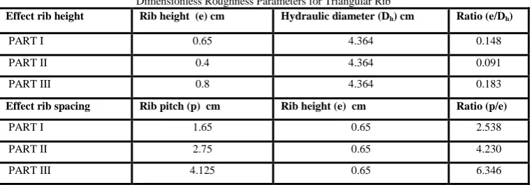
Numerical work is done by using computational fluid dynamics model through ANSYS FLUENT 15.0. Euler Lagrange multiphase- mixture model has used along with the k-ɛ turbulent model. This work is divided into three parts: PART I, II and III; the PART I which consider main part while the PART II deals with the studding effect of rib height by determining dimensionless roughness parameter, rib height to hydraulic diameter ratio (e/Dh). PART III deals with the studding effect of rib spacing by determining dimensionless roughness parameter, rib pitch to rib height ratio (P/e) to know the more effectiveness ribs with heat transfer. In PART I, had been modeled three-phase flow (water, gasoil and air) over triangle ribs in rectangular channel with constant rib height (e = 0.65 cm) and rib spacing (pitch, p =1.65 cm) as shown in figure (3) by using mixture model with different parameters depending on the test variables and relying on the experimental results to compare and validate the CFD results.PART II, had been modeled three-phase flow (water, gasoil and air) over triangle ribs in rectangular channel with variation rib height (e = 0.4 cm, 0.8 cm) and constant rib spacing (pitch, p = 1.65 cm) as shown in figure (4) by using mixture model also. PART III, had been modeled three-phase flow (water, gasoil and air) over triangle ribs in rectangular channel with constant rib height (e = 0.65 cm) and variation rib spacing

(pitch, p = 2.75 cm, 4.125 cm) as shown in figure (5) by using mixture model also. Table (2) explain dimensionless roughness parameters rib height to hydraulic diameter ratio (e/Dh) and rib pitch to rib height ratio (p/e).

3.1. Geometry Model and Boundary Conditions.

As shown in figure (3), Solid Work 2013 software used to modeling as a two-dimension structure for the three-phase flow system as a rectangle with lines represented as a ribs on the x-y plan with (3 cm) horizontal dimension and (70 cm) vertical dimension. After that, a surface was generated from the sketch. Entry region was divided to the thirteen sections, six sections for inlet water superficial velocity, six sections for inlet gasoil superficial velocity and one section for inlet air superficial velocity which is bigger from the other sections. Boundary conditions, from the bottom of the of the geometry, continuous phase (water) and dispersed phase (gasoil, air) superficial velocities enter with inlet phases temperature and volume fraction where these are taken from experimental data. Ribs region set as constant heat flux which is same the experimental value. The outlet of the geometry, was set to be outlet pressure and the right and left sides set as wall. The remaining portion of the left side and right side was set to be adiabatic wall.

Table II

Dimensionless Roughness Parameters for Triangular Rib

Effect rib height Rib height (e) cm Hydraulic diameter (Dh) cm Ratio (e/Dh)

PART I 0.65 4.364 0.148

PART II 0.4 4.364 0.091

PART III 0.8 4.364 0.183

Effect rib spacing Rib pitch (p) cm Rib height (e) cm Ratio (p/e)

PART I 1.65 0.65 2.538

PART II 2.75 0.65 4.230

PART III 4.125 0.65 6.346

(

" Qel loss)

A Q

q  



s

"



y

b

q

h

T



T

=





b in out in

T

Y

L

T

(5)

-IJMME -9 8 9 8 -705 4 17

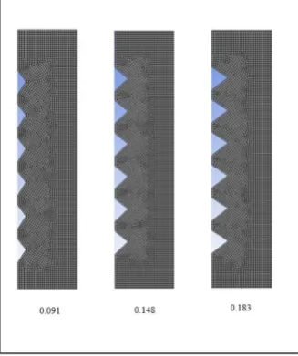
3.2 The mesh

In this work, the geometry of the rectangular channel with ribs was divided into small square element (Quadrilateral structured grid) using the Meshing combined with Ansys Workbench 15.0 with maximum and minimum size equal to (0.001 m) through fine span angle center and medium smoothing mesh. Figure (6, 7) depict mesh for three-phase system.

3.3. Problem Assumptions.

In order to simulate the three-phase flow with heat transfer model, the following assumptions were made.

1. Steady state two-dimensional fluid flow and heat transfer.

2. The flow is turbulent and incompressible. 3. Constant fluid properties.

4. Negligible radiation heat transfer, body forces and viscous dissipation.

5. Uniform heat flux. 6. No-slip boundary is applied at all walls of the

flow channel.

7. The gravity in y direction is (-9.81 m/s2_).

3.4. Governing Equations

The fundamental governing equations of fluid dynamics in the numerical work are continuity, momentum and energy equations in two dimensional. Mixture model solves the governing equations for each phase, a mixture model was used where the phases moved at different velocities. The general form of governing equations can be written from (Fluent User’s Guide, 2006)

1. Continuity Equation

(a)

(a) (b)

Fig. 7. The Mesh for Different Ratio (p/e) (b)

Fig. 3. Geometry for PART I Fig. 4. Geometry for PART II

(a) e= 0.4cm, (b) e= 0.8cm

Fig. 5. Geometry for PART III

(a) p = 2.75cm (b) p = 4.125cm

(6)

-IJMME -9 8 9 8 -705 4 17

The continuity equation was used to calculate the phase’s volume fraction. Because the volume fractions for all phases equals to one for that volume fraction of the primary phase was calculated through the summation

of the volume fraction of the secondary phases:

  

.

_m m



0

m

t







_

_



……….. (12)

Where



m_{is mass-averaged velocity is represented as:}

1

n

k k k

k m

m

  









..……… (13)

and



_m is the density of mixture:

1

n

m k k

k



 





_{……….. (14)}

k



is the volume fraction of phase k.

2. Momentum Equation

The momentum equation for the mixture can be obtained by summing the individual momentum equations for all phases. It can be expressed as:













, ,

1

.

m m m m m m m m

n k

m k dr k dr k k

t

g

F



_



_{ }



_







_{ }







_

_

 

    

_



 

_













   









…(15)

Where n is the number of phases ,

F

is a body force, and

m



is the viscosity of the mixture, which is given by:

1

n

k

m k

k











……….. (16)

Where

,

dr k



is the drift velocity for secondary phase k:

,

dr k

k

m











.……….. (17)

3. ENERGY EQUATION

The general form of this equation is given by:











1



1

.

_k

n n

k k

k k k k k

k k

eff

t

S





_{ }

 





_

_









 





(7)

-IJMME -9 8 9 8 -705 4 17

Where

_k

eff is the effective conductivity







k



k



k

t



, where

k

t is the turbulent thermal

conductivity. The first term on the right-hand side of Eq. (18) represents energy transfer due to conduction.

_S

_ includes any other volumetric heat sources. Also, in equation (18)

…...…... (19)

For an incompressible phase Ek= hk, where hkis the sensible enthalpy for phase k.

3.5. Turbulent Model

Ansys Fluent 15.0 exhibit three approaches for the k-epsilon

turbulence model in the multiphase flow

1. Turbulence mixture model 2. Turbulence dispersed model 3. Turbulence model for each phase

Depending on the deviation between experimental and numerical results, being choosing the turbulence K-ɛ standard mixture model was set for the three phases model which can be defined through these equations (Fluent User’s Guide, 2006).









,

.

t m

k m

m m m m

k

t

k

G







_











_

_

_

_

_

_

_







_

_

……….. (20)

 





,





1 , 2

.

t m _{k m}

m m m m

t

_

k

C G



C









_











_

_

_

_{ }

_

_







_

_

.……... (21)

Where ε is the turbulent dissipation rate, Gk is the generation of turbulence kinetic energy, and



is the turbulent Prandtl number for k and ε.

The density and the velocity of the mixture,



_m and m



, are computed as following:

1

n

i

m i

i











……….. (22)

1

n

i i i i

n m

i i i















……….. (23)

The turbulent viscosity,

,

t m



, and the production of turbulence kinetic energy,

G

__,_m, are computed as following:

2

,

t m m

k

C







_

……….. (24)

 

,m t m, m m

:

m

G















_



_









.……….. (25)

The model constants can be seen in table (3).

2

k k k

k

h

p

E





(8)

-IJMME -9 8 9 8 -705 4 17

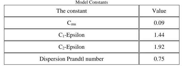
Table III Model Constants

The constant Value

Cmu 0.09

C1-Epsilon 1.44

C2-Epsilon 1.92

Dispersion Prandtl number 0.75

These default values have been determined based on experiments for fundamental turbulent three-phase flow.

4. RESULTS AND DISCUSSION 4.1. Heat Transfer Coefficient Results

4.1.1. Effect Water Superficial Velocity

Figure (8 a, b, c) show the effect of increasing water superficial velocity on the local heat transfer coefficient for three different values of water superficial velocity with various values of air superficial velocity and various values of heat flux with constant gasoil superficial velocity. It can be seen that the heat transfer coefficient profile increased with increasing water superficial velocity for all heat flux values. When the amount of water increases inside the channel, water superficial velocity increase for that the turbulence inside the test channel is increased and the mixing between phases (water, gasoil and air) being high, leading to increase in the heat transfer coefficient inside the test channel. The numerical results seemed to have the same influence as the experimental results with a deviation of about (2.092 % - 14.657 %) found between them.

4.1.2 Effect Gasoil Superficial Velocity

Figure (9 a, b, c) show the local heat transfer coefficient increased with gasoil superficial velocity increase with respect to the different values of water superficial velocity and constant air superficial velocity value for different values of heat flux. Also show a comparison between the experimental and numerical results at the same as the previous point in water effect case which created with the same coordinate where the temperature sensors situated experimentally. The numerical results seemed to have the same influence as the experimental results with a deviation of about (2.58% - 17.545%) found between them. When gasoil phase adds to the working fluid, velocity of working fluid is increase that’s lead to the heat transfer coefficient increase. The reason back to more increase for turbulence which create a vortex aid to high heat transfer from the rib surface to the working fluid.

4.1.3 Effect Air Superficial Velocity

The effect air phase showed in figure (10 a, b, c) which is illustrates the effect of increasing air superficial velocity on the local heat transfer coefficient results for various values of gasoil superficial velocity and heat flux with constant water superficial velocity. It is also, show a comparison between the experimental and the numerical results found at a same mentioned pervious point at case water and gasoil

effect. The numerical results seemed to have the same influence as the experimental results with a deviation of about (1.588 % -16.594 %) found between them. Adding air phase to the working fluid also aid to increase the working fluid superficial velocity by increase the turbulence generated by create bubbles which creates vortices around top surface of the triangular rib for that high heat transfer from the rib surface to the working fluid. For all figures (8,9,10) the temperature difference between the rib surface and mixture core is decreases at phase superficial velocity increase. Because the relation between temperature difference and phase superficial velocity is inversely proportional according to equation (7). The highest values of heat transfer coefficient were at effect water superficial velocity on heat transfer. because heat transfer coefficient is a function of the properties of the system such as geometry of the system and fluid regime and one of the factors which depends on it is physical property of the working fluid (three-phase flow) such as density (ρ) where the water density is bigger from the other fluids (gasoil and air).

4.2 Effect Rib on Heat Transfer Coefficient

(9)

IJENS © October 2017 IJENS -IJMME -9 8 9 8 -705 4 17

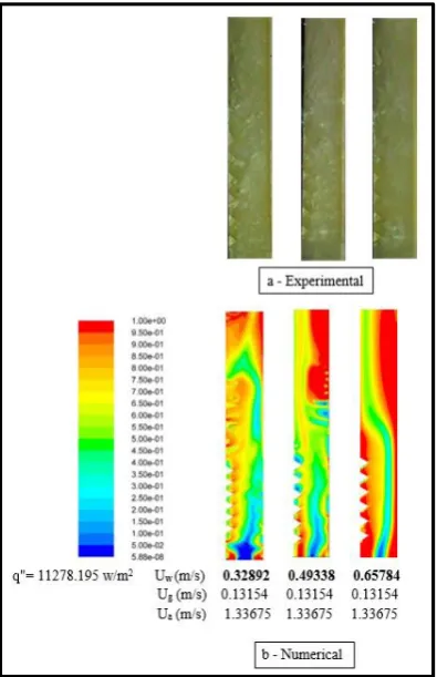
turbulence of flow in the channel then heat transfer increased as shown in figures (12) to (14). These figures show the experimental flow behavior through the photographs that were taken for test channel and visually compared it with the contour ofwater, gasoil and air volume fraction respectively found by numerical simulation. The rectangular channel fitted with triangular rib. The presence of this rib helps separate flow, for that a turbulence flow is higher, since separation causes local flow reversal, enhanced mixing, and thus more heat transfer. A close similarity for the behavior of flow between the experimental photos and the images of water, gasoil and air volume fraction found

with ANSYS FLUENT 15.0.The computational fluid dynamics simulation results depended on the superficial velocity of water, gasoil and air and heat flux input into the channel, the channel outlet mixture gage pressure, geometry and type of the ribs, and the volume fraction which gave a simulation results varied up and down the experimental results with a deviation as pervious mentioned. This is because, it was a changed phenomenon and controlled by different parameters that being assumed throughout these simulations, so those values can be changed by making different assumptions.

Fig. 8. Effect Water Superficial Velocity on Heat Transfer Coefficient (a) Uw=0.16446 m/s (b) Uw= 0.32892 m/s (c) Uw= 0.49338 m/s

(c)

1 1.5 2 2.5 3 3.5 4 4.5

Air Superficial Velocity (m/s)

0 500 1000 1500 2000 2500 3000 3500 4000 4500 5000 5500 6000 6500 7000 H ea t T ra n sf er C o ef fi ci en t (w /m 2k )

Uw= 0.32892 m/s Ug= 0.3963 m/s

11278.195 w/m2 13157.894 w/m2 15037.593 w/m2 Experimental Numerical

1 1.5 2 2.5 3 3.5 4 4.5

0 500 1000 1500 2000 2500 3000 3500 4000 4500 5000 5500 6000 6500 7000 H ea t T ra n sf er C o ef fi ci en t (w /m 2k ) Uw=0.49338 m/s Ug= 0.3963 m/s

11278.195 w/m2 13157.894 w/m2 15037.593 w/m2 Experimental Numerical 1 1.5 2 2.5 3 3.5 4 4.5

Air Superficial Velocity (m/s) 0 500 1000 1500 2000 2500 3000 3500 4000 4500 5000 5500 6000 6500 7000 H e a t T r a n sf e r C o e ff ic ie n t (w /m 2k )

Uw= 0.16446 m/s Ug= 0.3963 m/s

(10)

Fig. 9. Effect Gasoil Superficial Velocity on Heat Transfer Coefficient

Ug= 0.13154 m/s (b) Ug= 0.3963 m/s (c) Ug= 0.65772 m/s

(a) (b)

(c)

0.1 0.2 0.3 0.4 0.5 0.6 0.7 Water Superficial Velocity (m/s)

Ug= 0.13154 m/s Ua= 1.33675 m/s

0.1 0.2 0.3 0.4 0.5 0.6 0.7 Water Superficial Velocity (m/s)

0 500 1000 1500 2000 2500 3000 3500 4000 4500 5000 5500 6000 6500 7000 H ea t T ra n sf er C oe ff ic ie n t (w /m 2k )

Ug= 0.3963 m/s Ua= 1.33675 m/s

0.1 0.2 0.3 0.4 0.5 0.6 0.7

Water Superficial Velocity (m/s)

0 500 1000 1500 2000 2500 3000 3500 4000 4500 5000 5500 6000 6500 7000 H e a t T r a n sf e r C o e ff ic ie n t (w /m 2k )

Ug= 0.65772 m/s Ua= 1.33675 m/s

(11)

Fig. 10. Effect Air Superficial Velocity on Heat Transfer Coefficient

(a) Ua= 1.33675 m/s (b) Ua= 2.6735 m/s (c) Ua =4.01026 m/s

(c)

(a) (b)

0.1 0.2 0.3 0.4 0.5 0.6 0.7 Gasoil Superficial Velocity (m/s)

Ua= 1.33675 m/s Uw= 0.16446 m/s

Ua= 2.6735 m/s Uw= 0.16446 m/s

0.1 0.2 0.3 0.4 0.5 0.6 0.7

Gasoil Superficial Velocity (m/s)

0 500 1000 1500 2000 2500 3000 3500 4000 4500 5000 5500 6000 6500 7000 H e a t T r a n sf e r C o e ff ic ie n t (w /m 2k )

Ua= 4.01026 m/s Uw= 0.16446 m/s

(12)

-IJMME -9 8 9 8 -705 4 17

Fig. 11. stream lines for the turbulent intensity inside the channel

(13)

-IJMME -9 8 9 8 -705 4 17

Fig. 13. Contours of Gasoil Volume Fraction

(14)

-IJMME -9 8 9 8 -705 4 17

4.3. Temperature Distribution

4.3.1. Effect Water Superficial Velocity

Figure (15 a, b) shows the effect of water superficial velocity on the contours of temperature distribution inside the channel with triangular rib at constant values of gasoil and air superficial velocities and various values of heat flux, 0.1315 m/s, 1.3368 m/s and 11278.195 w/m2,_15037.593 w/m2_{respectively. As the superficial velocity of water} increased from 0.3289 m/s to 0.6578 m/s the temperature distribution decreased inside the channel. The reason for this effect was a result of increasing the superficial velocity of water and decrease the time residence of mixture inside the channel which caused an increase in the water flow rate and reduced the temperature difference along the channel according to Eq. (7).

4.3.2 Effect Gasoil Superficial Velocity

Figure (16 a, b) shows the effect of gasoil superficial velocity on the contours of temperature distribution inside the channel with triangular rib at constant values of water and air superficial velocities and various values of heat flux 0.6578 m/s, 1.3368 m/s and 11278.195 w/m2,_15037.593 w/m2_{respectively. As the superficial velocity of gasoil} increased from 0.1315 m/s to 0.6577 m/s the temperature distribution decreased as a temperature difference from

5.170 k˚ to 2.185 k˚ inside the channel. The reason for this effect was a result of increasing the superficial velocity of gasoil which aids to increase the mixture velocity and create a high turbulence but with percentage low from the water effect resulting different density and decrease the time residence of mixture inside the channel which caused an increase in the gasoil flow rate and reduced the temperature difference along the channel according to Eq. (7).

4.3.3 Effect Air Superficial Velocity

Figure (17 a, b) show the effect of air superficial velocity on the contours of temperature distribution inside the channel with triangular rib at constant values of water and gasoil superficial velocities and various values of heat flux, 0.3289 m/s, 0.1315 m/s and 11278.195 w/m2,_{15037.593 w/m}2 respectively. As the superficial velocity of air increased from 1.3368 m/s to 4.0103 m/s the temperature distribution decreased as a temperature difference from 5.332 k˚ to 2.891 k˚ inside the channel. At adding air to the mixture as a three phase, bubbles create and filled the channel which works to increase the turbulence, then improvement heat transfer but with percentage low from the water effect also resulting different density and decrease the time residence of mixture inside the channel which caused an increase in the air flow rate and reduced the temperature difference along

the channel according to Eq. (7).

Fig. 16. Effect Gasoil Superficial Velocity on Temperature Distribution Fig. 15. Effect Water Superficial

(15)

-IJMME -9 8 9 8 -705 4 17

5.EFFECT ROUGHNESS PARAMETERS

5.1. Effect of Rib Height

Figure (18 a) shows simulate separation mainstream at tip of the ribs as show in the figure, where the rib height is (0.4cm) with e/Dh= 0.091. As shown the flow separate only without create recirculation bubble which weaken the rate of heat transfer. While figure (18 b) shows simulate separation mainstream at tip of the ribs, where the rib height is (0.65cm) with e/Dh= 0.148. Also, as shown the flow separate only. Figure (18 c) show simulate separation mainstream at tip of the ribs, where the rib height is (0.8 cm) with e/Dh= 0.183. As shown the flow separate with create large recirculation bubble between the ribs.

Figure (19) display change heat transfer coefficient with change blockage ratio (e/Dh) from 0.091 to 0.183 at variation superficial velocity of water phase form 0.3289 m/s to 0.6578 m/s with constant gasoil and air superficial velocity 0.1315 m/s, 1.3368 m/s respectively, constant power 120 watt. From this figure observed the local heat transfer coefficient increased for all blockage ratio (e/Dh) values with keeping rib spacing constant (p =1.65cm). As well as, the highest values of local heat transfer coefficient were with lowest value of blockage ratio (0.091) which it means the rib height is 0.4cm. lowest values of local heat transfer coefficient were with highest value of blockage ratio (0.183) because at increase the blockage ratio the rib height increased and this leads to a larger recirculation area behind the rib (see figure 18 c).

Figure (20) represents change heat transfer coefficient with change blockage ratio from 0.091 to 0.183 at variation superficial velocity of gasoil phase form 0.1315 m/s to 0.6577 m/s with constant water and air superficial velocity 0.3289 m/s, 1.3368 m/s respectively, constant power 120 watt, with keeping rib spacing constant (p =1.65cm). From this figure observes. This figure explains, the local heat transfer coefficient increased for all blockage ratio (e/Dh) values. As well as, the highest values of local heat transfer coefficient were with lowest value of blockage ratio (0.091) but with lower values from figure (19). lowest values of local heat transfer coefficient were with highest value of blockage ratio (0.183) because to create recirculation region between the ribs which difficult mainstream (three phase flow) passing this area.

Figure (21) show change local heat transfer coefficient with change blockage ratio from 0.091 to 0.183 at variation superficial velocity of air phase form 1.3368 m/s to 4.0103 m/s with constant water and gasoil superficial velocity 0.3289 m/s, 0.1315m/s respectively, constant power 120 watt with keeping rib spacing constant (p =1.65cm). This figure offer, the local heat transfer coefficient increased for all blockage ratio (e/Dh) values. As well as, the highest values of local heat transfer coefficient were with lowest value of blockage ratio (0.091) but with lower values from figures (19,20). lowest values of local heat transfer coefficient were with highest value of blockage ratio (0.183) for the same reason in figures (19,20).

(16)

-IJMME -9 8 9 8 -705 4 17

Fig. 18. Comparison of Flow Fields in Ribbed Channel, Triangle Rib

With different Blockage Ratio (e/Dh).

0.3 0.4 0.5 0.6 0.7

1000 2000 3000 4000 5000 6000 7000

H

e

a

t

T

r

a

n

sf

e

r

C

o

e

ff

ic

ie

n

t

(w

/m

2k

)

Ug=0.1315m/s,Ua=1.3368 m/s e/Dh= 0.091 e/Dh= 0.148 e/Dh= 0.183

0 0.1 0.2 0.3 0.4 0.5 0.6 0.7

Gasoil Superficial Velocity (m/s)

1000 2000 3000 4000 5000 6000 7000

H

e

a

t

T

r

a

n

sf

e

r

C

o

e

ff

ic

ie

n

t

(w

/m

2k

)

Uw=0.3289 m/s,Ua=1.3368 m/s e/Dh= 0.091 e/Dh= 0.148 e/Dh= 0.183

Fig. 19. Effect Rib Height on Heat Transfer Coefficient with Different Water Superficial Velocity.

(17)

-IJMME -9 8 9 8 -705 4 17

5.2.Effect of Rib Spacing

Figure (22 a), mainstream is separates only from the surface due to the rib, as flow continuously, vortex develop immediately downstream of the ribs between of them. This area is produces hot fluid cells which gives heat transfer low from the other figures (22 b,c).

In figure (22 b) when the mainstream flow over the ribs, it separates from the rib surface at tip of triangular rib and reattaches at the point between the ribs producing high heat transfer from the figure (22 a).

In figure (22 c), at mainstream flow over the ribs, it separates from the rib surface at tip of triangular rib and reattaches to the region between the ribs with create recirculation bubble which if it bigger tends to reduce the heat transfer. This is an area of relatively high heat transfer from the other figures (22 a, b) due to impingement of the mainstream flow on the region between the ribs.

Figure (23) explains change local heat transfer coefficient with change rib pitch-to-height ratio (p/e) with various values of water superficial velocity from 0.3289 m/s to 0.6578 m/s, constant gasoil and air superficial velocity 0.1315 m/s, 1.3368 m/s respectively, and constant power 120 watt with keeping rib height constant (e = 0.65 cm). From this figure, the local heat transfer coefficient increases with increasing of rib pitch-to-height ratio from 2.538 to

6.346. Highest values for local heat transfer coefficient at rib pitch-to-height ratio 6.346 because of the wider rib spacing and accompanied by separation flow with reattachment point (see figure 22 c). Clearly, the smallest values for local heat transfer coefficient at 2.538 because of without reattachment point.

Figure (24) show change local heat transfer with change rib pitch-to-height ratio (p/e) with various values of gasoil superficial velocity from 0.1315 m/s to 0.6577 m/s, constant water and air superficial velocity 0.3289 m/s, 1.3368 m/s respectively, and constant power 120 watt with keeping rib height constant (e = 0.65 cm). From this figure, the local heat transfer coefficient increases with increasing of rib pitch-to-height ratio because of separation flow with reattachment point between two ribs.

In figure (25) represent change local heat transfer coefficient with change rib pitch-to-height ratio with variation of air superficial velocity form 1.3368 m/s to 4.0103 m/s, constant water and gasoil superficial velocity 0.3289 m/s, 0.1315m/s respectively, and constant power 120 watt with keeping rib height constant (e =0.65cm). From this figure, the local heat transfer coefficient increases with increasing of rib pitch-to-height ratio from 2.538 to 6.346

for the same reason in figures (23,24).

1 1.5 2 2.5 3 3.5 4 4.5

Air Superficial Velocity (m/s) 1500

2000 2500 3000 3500 4000 4500

H

ea

t

T

ra

n

sf

er

C

o

ef

fi

ci

en

t

(w

/m

2k

)

Uw=0.3289 m/s,Ug=0.1315 m/s e/Dh= 0.091 e/Dh= 0.148 e/Dh= 0.183

(18)

-IJMME -9 8 9 8 -705 4 17

0.2 0.3 0.4 0.5 0.6 0.7

1000 2000 3000 4000 5000 6000 7000

H

ea

t

T

ra

n

sf

er

C

o

ef

fi

ci

en

t

(w

/m

2k

)

Ug=0.1315 m/s,Ua=1.3368 m/s p/e=2.538 p/e= 4.230 p/e= 6.346

1000 2000 3000 4000 5000 6000 7000

H

e

a

t

T

r

a

n

sf

e

r

C

o

e

ff

ic

ie

n

t

(w

/m

2k

)

Uw=0.3289 m/s,Ua=1.3368 m/s p/e=2.538 p/e= 4.230 p/e= 6.346 Fig. 22. Comparison of Flow Fields in Ribbed Channel, Triangle Rib

With different Rib Spacing Ratio (P/e).

Fig. 23. Effect Rib Spacing on Heat Transfer Coefficient with Different Water Superficial Velocity.

(19)

-IJMME -9 8 9 8 -705 4 17

6. CONCLUSIONS

This work presented experimental and numerical study for heat transfer by forced convection and for temperature distribution in a vertical rectangular channel with triangular ribs for three-phase flow (water-gasoil-air) with uniform to 2 11278.195 w/m ranges from

heat flux which it

The following conclusions are drawn from .

2 15037.593 w/m

this work.

1- Experimentally and numerically, increasing the water superficial velocity from 0.3289 m/s to 0.65784 m/s, lead to improve local heat transfer coefficient by (48.5 %, 49.8 %) respectively with uniform heat flux 11278.195 w/m2_.

2- Experimentally and numerically, increasing the gasoil superficial velocity from 0.13154 m/s to 0.65772 m/s lead to improve local heat transfer

1 1.5 2 2.5 3 3.5 4 4.5

1500 2000 2500 3000 3500 4000 4500

H

ea

t

T

ra

n

sf

er

C

oe

ff

ic

ie

n

t

(w

/m

2 k)

Uw=0.3289 m/s,Ug=0.1315 m/s p/e = 2.538 p/e = 4.230 p/e = 6.346

1 1.5 2 2.5 3 3.5 4 4.5

Air Superficial Velocity (m/s) 1500

2000 2500 3000 3500 4000 4500

H

ea

t

T

ra

n

sf

er

C

oe

ff

ic

ie

n

t

(w

/m

2 k

)

Uw=0.3289 m/s,Ug=0.1315 m/s p/e = 2.538 p/e = 4.230 p/e = 6.346

Fig. 5.34. Effect Rib Spacing on Heat Transfer Coefficient With Different Gasoil Superficial Velocity.

(20)

-IJMME -9 8 9 8 -705 4 17

coefficient by (35.8 %, 36.1 %) respectively with uniform heat flux 11278.195 w/m2_.

3- Experimentally and numerically, increasing the air superficial velocity from 1.33675 m/s to 4.01026 m/s lead to improve local heat transfer coefficient by (20.1 %,18.0 %) respectively with uniform heat flux 11278.195 w/m2_.

4- Numerically, at decrease rib height to channel hydraulic diameter ratio (e/Dh) from 0.183 to 0.091 lead to improve local heat transfer coefficient by 51.7 % at increasing water superficial velocity from 0.3289 m/s to 0.65784 m/s with uniform heat flux 11278.195 w/m2_. 5- Numerically, at decrease rib height to channel

hydraulic diameter ratio (e/Dh) from 0.183 to 0.091 lead to improve local heat transfer coefficient by 50.1 % at increasing gasoil superficial velocity from 0.13154 m/s to 0.65772 m/s with uniform heat flux 11278.195 w/m2_. 6- Numerically, at decrease rib height to channel

hydraulic diameter ratio (e/Dh) from 0.183 to 0.091 lead to improve local heat transfer

coefficient by 22.9 % at increasing air superficial velocity from 1.33675 m/s to 4.01026 m/s with uniform heat flux 11278.195 w/m2_.

7- Numerically, at increase rib pitch to rib height ratio (p/e) from 2.538 to 6.346 lead to improve local heat transfer coefficient by 59.3 % at increasing water superficial velocity from 0.3289 m/s to 0.65784 m/s with uniform heat flux 11278.195 w/m2_.

8- Numerically, at increase rib pitch to rib height ratio (p/e) from 2.538 to 6.346 lead to improve local heat transfer coefficient by 54.2 % at increasing gasoil superficial velocity from 0.13154 m/s to 0.65772 m/s with uniform heat flux 11278.195 w/m2_.

9- Numerically, at increase rib pitch to rib height ratio (p/e) from 2.538 to 6.346 lead to improve local heat transfer coefficient by 25.2 % at increasing air superficial velocity from 1.33675 m/s to 4.01026 m/s with uniform heat flux 11278.195 w/m2_.

NOMENCLATURE SUBSCRIPTS Re: Reynold number. m: mixtrue U: velocity. m/s w: water

Dh: hydrodynamic diameter, m g: gasoil A: cross-sectional area, m2_{a: air}

W: wetted perimeter of the channel, m c: continuous phase h: heat transfer coefficient, w/m2_{k y: y- direction} T: temperature, kͦ s: rib surface q"_{: heat flux, w/m}2_{b: bulk temperature}

: electric power Y: position along stremwise : thermal losses in: entrance

m•: mass flow rate, kg/s out: outlet ∆T: temperature different

cp: specific heat at constant pressure, J/kg k Nu: Nusselt number

ʋ: mass averaged velocity, m/s U: Liquid superficial velocity m/s.

Q: Volume flow rate m3_/s.

GREEK SYMBOLS

μ: viscosity, kg/m. s

α:fraction of dispersed phase in liquid mixture ρ: density. kg/m3

REFERENCES

[1] Ansari M.R. and Arzandi B. “Two-phase gas–liquid flow regimes for smooth and ribbed rectangular ducts” International Journal of Multiphase Flow 38 (2012) 118–125.

[2] Asano, H., Takenaka, N., and Fujii, T., “Flow characteristics of gas–liquid two-phase flow in plate heat exchanger (Visualization and void fraction measurement by neutron radiography)”, Experimental Thermal and Fluid Science, Japan, V. 28, No. 2, PP. 223–230, 2004.

[3] AL-Turaihi R. S., “Experimental Investigation of Three Phase Flow (Liquid-Gas-Solid) In Horizontal Pipe”, International Journal of Innovative Research in Computer Science & Technology (IJIRCST).

[4] Fluent User’s Guide, “Modeling Multiphase Flows”, Fluent Inc.

September 29, 2006.

[5] Jaurker A. R., J. S. Saini, and B. K. Gandhi. "Heat transfer and

friction characteristics of rectangular solar air heater duct using

rib-grooved artificial roughness." Solar Energy 80.8 (2006):

895-907.

[6] Hanafizadeh P. , Shahani A. , Ghanavati A. , Behabadi M. A. “Experimental Investigation of Air‐Water‐Oil Three‐Phase Flow Patterns in Inclined Pipes” Experimental Thermal and Fluid

el

Q

(21)

-IJMME -9 8 9 8 -705 4 17

ScienceVolume 84, June 2017, Pages 286–298.ISSN: 2347-5552, Volume-4, Issue-4, July 2016.

[7] Lawrence C. Edomwonyi-Otu, Panagiota Angeli, “Pressure drop and holdup predictions in horizontaloil–water flows for curved and wavy interfaces”, Chemical Engineering Research and

Design, Cherd-1615, 2014. [8] Weisman, J., Lan, J., and Disimile, P., “Two-Phase (Air-Water)

Flow Patterns and Pressure Drop in The Presence of Helical Wire Ribs”, International journal of multiphase flow, Vol. 20,

No. 5, PP. 885-899, 1994. [9] Yuyuan, W., Yu, L., Liufang, C., and Changhai, S., “Boiling