Calibrating Camera Shake Photographs Using Parallel
De-Convolution
Ahmed Sameh*, and Nazzly El Shazzly**
“Department of Computer and Information Systems Prince Sultan University, P.O.Box 66833 Riyadh, KSA 11586
**Department of Computer Science & Engineering, The American University in Cairo, P.O.Box 2511, Cairo, Egypt 11552
Contact Email: [email protected]
Abstract-- Camera shake causes images to be blurry. There are many techniques to de-blur an image. The process of removing image blur is called de-convolution. There are many different techniques for performing the de -convolution of images. In this paper, we propose a parallel de-blur algorithm inspired by Fergus et al. in [1]. The algorithm is performed by first estimating the blur kernel, then de -convolving the blurred image with that kernel in order to obtain the original clear image. The proposed parallel algorithm has a run time of O(log N). The algorithm is verified and tested.
1. INT RODUCT ION
Camera shake leads to motion blur in photographs. Removing that motion blur is an important procedure for digital photography and many other applications . Camera shake is modeled as a blur kernel convolved with the original image. Removing the blur is called image de-convolution. There are blind and blind image de-convolution techniques. In non-blind image de-convolution, the blur kernel is assumed to be known. The task of such an algorithm is to estimate the un -blurred image, called the latent image. Some traditional non-blind de-convolution methods are widely used today, such as Wiener filtering [7] and the Richardson-Lucy (RL) de-convolution [8]. The Richardson-Lucy de-de-convolution is used in this paper. In blind de-convolution, both the blur kernel and the latent image are assumed unknown. Such algorithms use probabilistic methods to obtain the latent image.
The algorithm that this paper presents is a blind de-convolution technique. It is inspired by Fergus et al. [1], which in turn builds upon the work of Miskin and MacKay [7]. It mainly adopts a Bayesian approach to find the blur kernel, and then reconstructs the image using the Richardson-Lucy de-convolution algorithm.
2. RELAT ED WORK
A lot of work is being done on image blurring or convolution. Many blind as well as non -blind image de-convolution algorithms exist. Yuan et al. [3] propose a non-blind image de-convolution algorithm that reduces ringing. Their approach is based on a new approach called bilateral Richardson-Lucy (BRL) that uses a multi-scale technique to recover the image. The multi-scale technique uses the image
reconstructed, at one iteration, as a guide in the next iteration. Ishiara and Komatsu [4] introduce a blind de-convolution method that deals with truncated images that are difficult to treat with conventional blind de-convolution algorithms. Trifas et al. [5] focus on the enhancement of medical images. They use a multi-resolution method to de-blur the image. Shan et al. [2] introduced a new algorithm for removing motion blur using a probabilistic model. They propose a unified model for both blind and non-blind de-convolution.
Also, some work has been done on parallel de-convolution algorithms. Matson and Borelli [6] introduced a parallelization of the PCID algorithm, which is a blind de-convolution algorithm.
3. IMAGE MODEL
The presented algorithm takes a blurred image B as input. It is assumed that the image B has been generated by the convolution of a blur kernel K with the latent (original) image L plus a noise factor N. The goal is to recover L from B without having any prior knowledge of the kernel K.
B = K ⊗L + N
where ⊗ denotes image convolution.
4. SEQUENT IAL ALGORIT HM
The sequential algorithm consists of two main steps. First, the blur kernel is estimated using an inference technique introduced by Miskin and MacKay [7]. Then, a standard de-convolution algorithm, Richardson-Lucy non-blind de-convolution, is applied.
The algorithm takes four user-specified inputs:
1. the blurred image B
2. a rectangular patch within the image 3. the maximu m resolution of the blur kernel
4. an initial guess to the orientation of the blur (vertical or horizontal)
gamma-correction with γ = 2.2. Gamma gamma-correction is a transformation technique used in image processing. It is a nonlinear operation for coding and decoding luminance (RGB values) in a still image. It is defined by the following power law transformation
Vout = Vinγ
Next, the input image B is converted to gray scale in order to estimate the blur kernel. A rectangular patch P within the image (specified by the user) is used to estimate the blur kernel. Using the blurred path P, the kernel K is estimated as well as the latent patch Lp. The optimizations are performed
on the gradients of P and Lp. The noise is assumed to have a
Gaussian distribution.
The algorithm varies the image resolution from coarse-to-fine. This is done to avoid local minima. At the coarsest level, the kernel is 3 x 3. It is initialized to one of two simple patterns, horizontal or vertical, which is specified by the user. The initial estimate for the latent gradient image is then produced using the estimated 3 x 3 initial kernel. The kernel is then recursively refined (i.e. its resolution is increased) until the full resolution kernel is achieved. The full resolution kernel’s size is also specified by the user. The values of K and the gradient of Lp produced at each level are used as an
initialization for the next level.
The inference algorithm runs on a small user selected patch in the image (see images in Appendix A). This is faster than using the entire image to infer the kernel. The patch is manually selected by the user. Manual selection of the patch is advantageous to an automatic selection, because it allows the user to avoid areas of saturation or uniformity that would not be very useful for the algorithm.
The size of the blur kernel affects the performance of the algorithm. Small blurs cannot be resolved if the kernel is too large; large blurs will be cropped if a very small kernel is used.
The initial estimate of the blur kernel, which is specified by the user to be either horizontal or vertical, helps the algorithm converge faster. However, the algorithm will produce the correct result either way.
At the next stage, the inferred kernel K is used to reconstruct the latent image L using Richardson-Lucy (RL) algorithm. The RL algorithm is an iterative non-blind de-convolution algorithm. The Richardson-Lucy algorithm reconstructs the original image by iteratively updating the image using the following equation:
It+1 = It [K*
K
tI
B
],
where It is the image at time t and It+1 is the image at time t + 1. K* is the adjoint of K.
The RL algorithm is an efficient algorithm for image de-convolution. It performs two convolutions and two multiplications per iteration. The authors of the algorithm recommend ten RL iterations to construct the image. For large blur kernels, it is recommended to increase the number of iterations. Matlab’s implementation of the RL algorithm (function name: “de-convlucy”) is used for this step.
The output of the RL method is then gamma-corrected to produce the final output image.
4.1 Performance Analysis
Four experiments have been conducted in order to analyze the sequential algorithm. The experiments have been done on two images using different settings for the maximum kernel resolution. A description of the experiments follows:
1. Image 1:
Original image size: 1600x1200 Maximum kernel resolution: 35x35
Experiment 1: Image was scaled to half its size by the algorithm before processing (800x600)
Experiment 2: Algorithm was run on the full resolution image
2. Image 2:
Original image size: 1024x1280 Maximum kernel resolution: 25x25
Experiment 1: Image was scaled to half its size by the algorithm before processing (512x640)
Experiment 2: Algorithm was run on the full resolution image
The Matlab profiler was used to obtain statistics about the algorithm while it is running. The output of the profiler consists of the total CPU time as well as the number of calls of each function, the calling functions and the child functions .
The functions in which the algorithm spent most of its time are as follows:
1. train_ensemble_main6: used in the inference of the kernel
2. train_ensemble_evidence6: used in the inference of the kernel
3. train_blind_deconv: used in the inference of the kernel
4. fft2: the Fast Fourier Transform of an image
5. ifft2: the Inverse Fast Fourier Transform of an image 6. de-convlucy: the de-convolution using the RL
algorithm
The function train_ensemble_main6 calls the function
train_ensemble_evidence6, which in turn calls
Transform to perform its calculations. It makes around 99% of the calls to the fft2 and the ifft2 functions (19136 calls out of 19157 total calls in one experiment).
The following table compares the number of calls and the CPU time of both the fft2 and the ifft2 functions in all experiments.
512x640 800x600 1024x1280 1600x1200
# Calls
CPU Time
# Calls
CPU Time
# Calls
CPU Time
# Calls
CPU Time fft2 16067 96 19157 1273 16595 476 24405 4379
ifft2 16058 125 19147 1488 16586 574 24395 5024
As observed from the data, the algorithm spends a lot of time calculating the Fast Fourier Transform and its inverse. The complexity of the sequential Fast Fourier Transform is O(N
log N) for N points. The algorithm of the Fast Fourier Transform is parallelizable. The ideal parallel time complexity would be O(log N). This provides a good opportunity for parallelism. If a parallel FFT algorithm was used instead of the sequential algorithm, the total CPU time of the de-blurring algorithm could be reduced considerably.
Another good opportunity for parallelism is the RL de -convolution. The de-convlucy function, which performs the RL algorithm, is called once in each run. The total CPU time of this function increases when the image resolution increases (see Table and figure).
512x640 800x600 1024x1280 1600x1200 CPU Time
(sec) 23 58 101 486
5. PARALLEL ALGORIT HM
According to the analysis results of the sequential algorithm, two experiments are conducted. The first experiment is conducted by replacing the FFT algorithm by its parallel equivalent. The CPU time of the algorithm is measured. The
second experiment introduces a parallelization of the RL algorithm.
The experiments are conducted using Matlab. Parallel algorithms are implemented using the MatlabMPI and the
pMatlab libraries developed for Matlab in the Massachusetts Institute of Technology (MIT) [9].
A brief introduction to the MatlabMPI and the pMatlab
libraries is given in the next section, followed by a description of the experiments.
5.1. MatlabMPI and pMatlab Libraries
MatlabMPI and pMatlab are libraries that enable parallel programming in Matlab. They were developed at the MIT Lincoln Laboratory [9][10].
MatlabMPI is an implementation of the Message Passing Interface (MPI) standard. It uses Matlab’s file I/O to perform communications. Standard MPI functions can be used, such as
MPI_Send to send a message, MPI_Recv to receive a message and MPI_Run to start a parallel process.
pMatlab is a library that provides a model for Global Array Semantics in Matlab. It makes use of the MatlabMPI library to encapsulate the communication layer and hide the implementation details from the developer. The developer defines the global array and how it should be divided among the processors in the program. The pMatlab array is responsible for re-distributing the actual data among processors.
To implement global arrays in Matlab, pMatlab introduces a new data type called the Distributed Matrix (dmat). In order to distribute the dmat object among processors the developer has to specify a map object and apply it to the Distributed Matrix. The map object specifies four parameters:
1. Grid: a vector of integers that specifies how each dimension of the matrix will be distributed among the processors
2. Distribution: there are three types of distributions: Block: each processor gets a contiguous
block of data (default)
Cyclic: data are interleaved among processors
Block-cyclic: contiguous blocks are interleaved
3. Processor list: specifies the ranks of the processors that work on each block
4. Overlap: specifies the amount of overlap between processors in each dimension. This option would be useful when parallelizing image processing algorithms such as convolution
5.2. Limitations of MatlabMPI and pMatlab To run a MatlabMPI process a script is used that is given the extension of the .m file to run on multiple nodes. This does not allow the .m file to take input arguments. To pass arguments RL Algorithm
0.00 100.00 200.00 300.00 400.00 500.00 600.00
512x640 800x600 1024x1280 1600x1200
Image Size
C
P
U
Ti
m
e
(
s
e
c
to the parallel algorithm, file I/O has to be used. Inputs are written to a .mat file before the parallel process is called. When a parallel process finishes, it writes its output to another file, which is read by the sequential part of the algorithm. This introduces some overhead in the overall performance. Another option would be the parallelization of the whole algorithm. This includes converting all the matrices into dmat objects and letting the master process work on the sequential part and the slaves do the parallel work as necessary.
5.3. Experiments
5.3.1 Experiment 1: The FFT algorithm
The FFT algorithm is implemented using pMatlab [11]. To obtain the FFT of an image, the two dimensional Fourier Transform must be used. The two dimensional Fourier Transform is obtained by applying the Fourier Transform in each dimension, once on the columns and then on the rows. To get the FFT of the rows, the matrix is first transposed. The second FFT operation is then applied to the transpose. The one-dimensional Fast Fourier Transform is overloaded in the
pMatlab library for the dmat object.
The code for the parallel FFT is shown below. The image is stored in the array pfftX, which is read from a file produced by the caller of the FFT process . The first map object is used to get the FFT on the columns, and the second map is used to get the FFT on the rows. The second map simulates the transpose of the first map. Assuming that 8 processors will be used in this experiment, the first map takes the first four processors and the second map uses the second set of processes. Block distribution will be used, i.e. the matrix is distributed in contiguous blocks among the processors. The result of the two FFT operations is aggregated in the master process and combined into one matrix, pfftZ. This is done automatically by
pMatlab when the agg() function is called.
% 1. read variables from file (pfftX) load('tmp_parallel_fft2');
% MxN Matrix size
M = size(pfftX,1); % rows N = size(pfftX,2); % columns
% Turn parallelism on or off. PARALLEL = 1;
% Initialize pMatlab. pMatlab_Init;
Ncpus = pMATLAB.comm_size; Hcpus = Ncpus / 2;
my_rank = pMATLAB.my_rank;
% Create Maps. map1 = 1; map2 = 1; if (PARALLEL)
% Break up channels.
map1 = map([1 Hcpus], {}, 0:Hcpus-1 ); map2 = map([Hcpus 1], {}, Hcpus:Ncpus-1 ); end
% Allocate data structures. A = zeros(M,N,map1); A(:,:) = pfftX; B = zeros(M,N,map2); C = zeros(M,N,map2);
% 2D fft
B(:,:) = fft(A, [], 1); % columns C(:,:) = fft(B, [], 2); % rows
pfftZ = agg(C);
if(my_rank == pMATLAB.leader)
save('tmp_parallel_fft2_out', 'pfftZ'); end
% Finalize the pMATLAB program pMatlab_Finalize;
5.3.2 Experiment 2: The RL algorithm
In this experiment, a parallelization of the Richardson-Lucy algorithm (see equation in Section 4) is implemented using
for its = 1:LUCY_ITS
%a. Convolution: IK=I x K
IK(:,:,1) = conv2(I_local(:,:,1), blur_kernel, 'same');
IK(:,:,2) = conv2(I_local(:,:,2), blur_kernel, 'same');
IK(:,:,3) = conv2(I_local(:,:,3), blur_kernel, 'same');
%b. Division: BIK=B/IK
BIK(:,:,1) = B_local(:,:,1) ./ IK(:,:,1); BIK(:,:,2) = B_local(:,:,2) ./ IK(:,:,2); BIK(:,:,3) = B_local(:,:,3) ./ IK(:,:,3); %c. Convolution: C = adjK x BIK
C(:,:,1) = conv2(BIK(:,:,1), adjK, 'same'); C(:,:,2) = conv2(BIK(:,:,2), adjK, 'same'); C(:,:,3) = conv2(BIK(:,:,3), adjK, 'same'); %d. Multiplication: I = I * C
I_local(:,:,1) = I_local(:,:,1) .* C(:,:,1); I_local(:,:,2) = I_local(:,:,2) .* C(:,:,2); I_local(:,:,3) = I_local(:,:,3) .* C(:,:,3);
end
I = put_local(I, I_local);
% 4. aggregate image and write output to file out = agg(I);
6. EXPERIMENT S AND RESULT S
This section demonstrates the experiments done on the images while varying the number of processors. The CPU times and communication times are measured to allow for a comparison between the performance of the sequential implementation and the parallel implementation.
6.1. Experiment 1: The FFT algorithm
This experiment is conducted on an image of size 512 x 640. To implement the 2D-FFT using pMatlab, two sets of processors need to be used, one for each dimension. For example, if 4 CPUs are used, the first dimension (e.g. columns) is divided among two processors (CPU 0 and CPU 1). The result is then redistributed among the second set of processors (CPU 2 and CPU 3) such that it represents the transpose of the previous result, on which the second dimension FFT is performed.
The following configurations are used in the experiments:
- 4 CPUs: 2 – 2 block distribution - 8 CPUs: 4 – 4 block distribution
The results compare the CPU time of one call to the parallel FFT to one call to the sequential FFT. The following table illustrates the results:
1 CPU 4 CPUs 8 CPUs Comp. Time (sec) 80.006 0.165 0.213 Comm. Time (sec) 0 64.687 35.179
2D FFT is a communication-intensive parallel computing task. The pMatlab and MatlabMPI abstract the hardware
architecture and system details. They both abstract the parallel data and task distribution through maps. The single CPU is fast enough for small datasets, but the time to
completion becomes significant as the number and size of FFT’s increase. We have followed the FFT pMatlab implementation found in [11]. Each processor will have the FFT results of its local dat. The data on other processors will need to be communicated to this processor if required for a subsequent stage of computation.
As it can be observed, the communication time decreases when the number of CPUs increases as the matrix size is considerably smaller. Also note that in addition to the computation time, the following steps introduce even more overhead:
1- Saving the input and output to file: It takes around 0.1 seconds each. This will increase with image size. 2- Initializing the MatlabMPI and pMatlab libraries and
starting the processes: around 6 seconds .
The optimized 2D FFT parallel algorithm in the Matlab library provides an overall better performance than the sequential algorithm. Although the parallelization of specific functions introduces a lot of overhead due to communication and file I/O, it is beneficial to parallelize the FFT function specifically.
6.2. Experiment 2: The RL algorithm
This experiment is conducted on an image of size 512 x 640 using 2, 4 and 8 CPUs. The image has been divided among the processors as follows:
- 2 CPUs:
o Block distribution
o Overlap: calculated from the size of the kernel, e,g, if the kernel is 25x25, then we have 12 overlapping pixels.
o The image has been divided horizontally among two processors
- 4 CPUs:
o Block distribution
o Overlap: calculated from the size of the kernel, e,g, if the kernel is 25x25, then we have 12 overlapping pixels.
o The image has been divided horizontally and vertically among two processors in each dimension
- 8 CPUs:
o Block distribution
o The image has been divided horizontally among four processors and vertically among twp processors
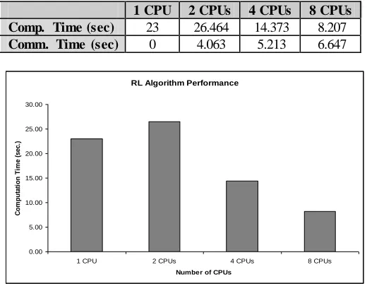
The following table illustrates the results:
1 CPU 2 CPUs 4 CPUs 8 CPUs Comp. Time (sec) 23 26.464 14.373 8.207 Comm. Time (sec) 0 4.063 5.213 6.647
As can be observed from the data the computation time decreases as the number of processors increases. Communication time increases as the number of processors increases. The overall performance is improving when using 4 or more CPUs. However, when using two CPUs, there is actually a slight increase in performance. Computation time is almost the same, but the overhead of communication degrades the performance. Communication and computation time are very close when using 8 CPUs. It is also noteworthy that it takes an average of 4.5 seconds to initialize the MPI environment on all processors and start the processes.
7. CONCLUSIONS
In this paper, we have introduced and implemented a parallelization for an algorithm to remove motion blur. Two experiments have been conducted. The first was replacing the FFT sequential function with a parallel algorithm, seeing as it is used extensively in the program. This experiment has proved to be beneficial even as it introduces lots of overhead. The second experiment is the parallelization of the Richardson-Lucy algorithm, which resulted in a slight speedup of the process. The two combined have achieved a run time speedup of O(log N)over the original sequential algorithm.
REFERENCES
[1] Rob Fergus, Barun Singh, Aaron Hertzmann, Sam T . Roweis, and William T . Freeman, “ Removing Camera Shake from a Single Photograph”, ACM SIGGRAPH 2006
[2] Qi Shan, Jiaya Jia and Aseem Agarwala, “ High-quality Motion De-blurring from a Single Image”, ACM SIGGRAPH 2008 [3] Lu Yuan, Jian Sun, Long Quan and Heung-Yeung Shum,
“Progressive Inter-scale and Intra-scale Non-blind Image De-convolution”, ACM SIGGRAPH 2008
[4] Nobuhito Ishiara and Shinichi Komatsu, “ Blind Recovery of T runcated Blurred Image Using Adaptive Masking Method”, Proceedings of the Winter International Sym posium on Inform ation and Com m unication Technologies, 2004
[5] Monica A. T rifas, John M. Tyler and Oleg S. Pianykh, “ Applying Multi-resolution Methods to Medical Image Enhancement”,
Proceedings of the 44th annual Southeast Regional Conference
ACM-SE 44, 2006
[6] Charles L. Matson and Kathy Borelli, “ Parallelization and Automation of a Blind Deconvolution Algorithm”, HPCMP Users Group Conference, June 2006
[7] Miskin, J., and MacKay, D. J. C., “ Ensemble Learning for Blind Image Separation and De-convolution”, Adv. in Independent Com ponent Analysis,M. Girolani, Ed. Springer-Verlag, 2000 [8] Richardson, W., “Bayesian-based iterative method of image
restoration”, Journal of the Optical Society of Am erica A 62, 55.59, 1972.
[9] Hahn Kim and Albert Reuther, “Writing Parallel Parameter Sweep Applications with pMatlab”, MIT Lincoln Laboratory, 2007 [10] Nadya T ravinin, Henry Hoffmann, Robert Bond, Hector Chan,
Jeremy Kepner and Edmund Wong, “pMapper: Automatic Mapping of Parallel Matlab Programs”, MIT Lincoln Laboratory, 2008
[11] Mullen J., Bliss N., Bond R., Kepner J., and Kim H., “High Productivity Software Development with PMatlab”, IEEE Scientific Programming Journal, V. 23, No. 1, January/February, 2009.
Fig. 1. Blurred image with user selected patch
Fig. 2. Inferred Kernel (greyscale)
Fig. 3. Latent Image
RL Algorithm Performance
0.00 5.00 10.00 15.00 20.00 25.00 30.00
1 CPU 2 CPUs 4 CPUs 8 CPUs
Number of CPUs
C
om
pu
ta
ti
on
Ti
m
e
(
s
e
c