HIGH PERFORMANCE WIRELESS COMMUNICATION CHANNEL USING LEACH
PROTOCOLS
Ch.Usha Kumari and M. Ramya Krishna
Department of E.C.E., Gokaraju Rangaraju Institute Engineering and Technology, Hyderabad, India [email protected], [email protected]
ABSTRACT
Wireless sensor networks take wide range of practical and useful applications. But there are many critical problems for efficient operations of sensor networks in real time applications. Sensor networks contain of number of nodes but with limited battery power and also wireless communications are deployed to collect useful information from the sensor node. It is very difficult for the sensor network to operate for a long period in an energy efficient manner for gathering sensed information. Energy saving is one critical issue for sensor networks since most sensors are equipped with non-rechargeable batteries that have limited lifetime. The power resource of each sensor node is limited. In this paper, we propose minimizing energy dissipation and maximizing network lifetime which is very important issue in the design of routing protocols for sensor networks. This paper we propose a new improved cluster algorithm of LEACH (Low Energy Adaptive Clustering Hierarchy) protocol which is intended to balance the energy consumption of the entire network and extend the lifetime of the network.
Keywords— Wireless Sensor networks, Clustering,LEACH, Energy efficiency, Low latency.
I. INTRODUCTION
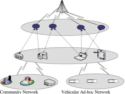
Wireless Sensor Networks (WSNs) are being used in wide range of possible applications such as environment monitoring, military operations, target tracking and surveillance system, vehicle motion control, earthquake detection, patient monitoring systems, pollution control system etc. These networks consist of SNs (sensor nodes) which are capable of monitoring and processing the data from a geographical location and send the same to remote location which is called as Base Station(BS). WSNs typically consist of small and inexpensive devices that communicate among each other using a multi hop wireless communication. Each node of WSN is called as a SN (sensor node) which contains one sensor, limited memory, low-power radio, embedded processors and is normally operated with battery. Each SN is responsible for sensing a desired event locally and for relaying a remote event sensed by other SNs so that the event is reported to the destination through BS. Sensor nodes have limited energy so applications and protocols for wireless sensor networks should be care-fully designed for optimized utilization of energy for longer network lifetime. Fig.1 shows the generalized view of wireless sensor networks, consists of a BS, Cluster Heads(CHs) and sensor nodes (SNs) deployed in a geographical region.
Community Network Vehicular Ad-hoc Network Fig 1 Wireless Sensor Network
Clustering is used in sensor networks for designing various energy efficient protocols. The important protocols used in this WSNs is LEACH (Low Energy Adaptive Clustering Hierarchy) [1]. It is a self-organi-zing clustering protocol which uses constant energy distribution among the sensor nodes in the network. The operation of this protocol is distributed into rounds and each round is distributed into two phases i.e. setup phase and steady-state phase.
Steady-state phase is always very long when compared to the set-up phase. In this protocol, the nodes organize themselves into local clusters. In this one node acts as a leader we call as cluster head and remaining nodes act as normal nodes. To increase the life time of the WSN, this protocol includes random rotation of the cluster heads and executes local data synthesis to transmit the amount of data from CHs to the BS. If BS is very far from the network, then the energy of cluster heads will be affected as only CHs are directly commu-nicating with the BS. Set of clusters will be different for different time interval and the decision to become a cluster head depends on the amount of energy left at the sensor node [3,4,7].
A. Radio Energy Dissipation model:
We have taken a simple model for energy pation in hardware radio where the transmitter dissi-pates energy to the power amplifier and radio electro-nics. The receiver dissipates energy to run the radio electronics [5,6,11,12]. Depending on the distance between the TX and RX, both the free space (fs) and multi path fading (mp) channel models are used.
If the distance is lesser than threshold, free space model is considered. Otherwise multi path model is considered. Therefore, to transmit a l-bit message a
distance d, the radio expends:
)
,
(
)
(
l
E
l
d
E
E
T
Tele
Tampf………… (1)
o o
mp ele
fs ele T
d
d
d
d
d
l
lE
d
l
lE
E
42
mp fs
d
0 ……….. (3)
The energy depends on many factors like
filtering, digital coding, spreading and modulation of the signal whereas the amplifier energy depends on
distance to the Eele receiver and the tolerable bit error
rate. The l-bit message, send over a distance is,
ele ele
R
R
l
E
l
lE
E
(
)
_(
)
…………
(4)
II. LEACHPROTOCOL
LEACH is a hierarchical cluster routing protocol for WSN which divides the nodes into clusters, in each cluster a particular node with extra privileges called CH is responsible for creating and manipulating a TDMA (Time division multiple access) schedule and sending aggregated data from nodes to the BS where these data
is needed using CDMA (Code division multiple access)
[8,18,19,20]. Remaining nodes are cluster members. The operation of LEACH is divided into rounds [13,14]. Each round begins with a set-up phase when the clusters are organized, followed by a steady-state phase when data are transferred from the nodes to the cluster head and on to the BS.
A. Set up phase
Every node decides independent of remaining nodes if they will become a cluster head or not. This choice considers when the node functioned as a cluster head for the last time (the node that not a cluster head for long time is more likely to chosen itself than nodes that have been a cluster head newly).
In the succeeding advertisement phase, the cluster heads inform their nearby nodes with an advertisement packet that they become cluster head. Non-cluster head nodes receive the advertisement packet with the heavy-duty received signal strength. Centred on all messages received in the cluster, the cluster head creates a TDMA (Time Division Multiple Acess) schedule, choose a CSMA code randomly, and announce the TDMA table to all nodes in the cluster [9,10,22]. After that steady-state phase starts.
B. Steady state phase
Data transmission begins in this phase. All nodes send their data in their allocated TDMA slot to the cluster head. This transmission uses a minimum amount of energy (pick based on the received signal strength of the cluster head advertisement). The radio of every non-cluster head node could have turned off until the nodes allocated TDMA slot, thus reducing energy dissipation in these nodes [16,17]. When whole data has been received, the cluster head cumulates data and send it to the base station. LEACH can achieve local accumulation of data in every cluster to minimize the amount of data that has transferred to the base station.
C. Cluster Head Selection Algorithm
LEACH forms clusters by means of a distributed algorithm, where nodes make independent decisions without any centralized control. Our objective is to design a cluster formation algorithm such that there are a definite number of clusters, K, during each round
[15]. Moreover, if nodes originate with equal energy, our aim is to try to evenly allocate the energy load amid all the nodes in the network so that there are no overly-utilized nodes that will run out of energy before the others. Being as a cluster head node is much more energy concentrated than being a non-cluster head node, this requires that every node take its chance as cluster head [2].
Each sensor selects itself to be a cluster head at the start of round r+1 (which begins at time t) with
probability pi(t).pi(t) is selected such that the expected
number of cluster heads for the round is K. Thus, if there are nodes in the network [21].
pi(t) = Probability that every sensor i picks itself to be
a cluster head at the stating of the round(r+1) at time t. N = no. of nodes in the network
N-K = normal nodes
Expected no. of cluster heads k = sum of probabilities of all sensors
N
i t p
k i
1 1 )
( …………. (5)
) (t
Ci = The indicator function determining whether or
not node i has been a cluster head in the most recent rounds
k N
r mod = most recent rounds
Where
k
N = nodes per cluster and r = no. of rounds
)
(
t
C
i = 0 means i is cluster head) (t
Ci = 1 means I is not a cluster head
rounds recent most in heads cluster
not are that nodes of no. Expected
head cluster of
no. Expected )
( P
i t
0
)
(
1
)
(
0
)
(mod
*
)
(
t
C
t
C
k
N
r
k
N
k
t
P
i i
i ……. (6)
Total no. of nodes that are eligible to be a cluster head at time t and energy is
)
(mod
*
)
(
k
N
r
k
N
t
C
E
N
i
i
………. (7)
N
i i t
P CH
E
1
1 * ) (
N
i
i i t C t P
1
) ( * ) ( E[CH]
k
k
N
r
k
N
k
N
r
k
N
k
CH
E
*
[
*
(mod
)]
)
(mod
*
]
[
… (8)If
E
i(
t
)
= node energy)
(
t
E
total = the aggregate remaining energy in the
,
1
)
(
)
(
min
)
(
k
t
E
t
E
t
P
total i i ………(9)
N i itotal t E t
E
1 ) ( )
( ………. (10)
The nodes with higher energy are more likely to become cluster head than nodes with less energy
The expected no. of cluster nodes is
k k t E t E t E t E t P CH E N i total N total
i
1 1 ) ( ) ( ... ) ( ) ( 1 * ) ( ][ … (11)
To use the probabilities in (9), every node must have an approximation of the total energy of all nodes in the wireless sensor network. This needs a routing protocol that allows every node to determine the total energy, whereas the probabilities in (6) enable every node to make completely independent decisions. One method to avoid this may be to estimate the cumulative node energy by multiplying the average energy of the nodes in every cluster by N. Note that to calculate the probabilities in (6) and (9) needs that each node knows the parameters K and N.
The optimal number of clusters K is a function of the number of nodes N circulated all over the region MxM of space. So, the nodes only need to find N assuming there is a predefined arrangement for M. To do this, all nodes can send “hello” messages to all their neighbors within a prearranged number of hops (to approximate M). Each node can sum the number of “hello” messages it receives—this is that node’s evaluation for the desired number of clusters can then be determined centered on these parameters. This approach allows LEACH to adapt to changing networks at the cost of increased overhead.
D. Energy Consumption Analysis
If l-bit message is transmitted over a distance d, then
Transmitted energy
E
T
E
Tele(
l
)
E
Tampf(
l
,
d
)
o o mp ele fs ele Td
d
d
d
d
l
lE
d
l
lE
E
4
2
If the distance d < a threshold d0 ……….. for Free
space (fs) model is used.
If the distance d ≥ a threshold d0 ………. for
Multipath (mp) model is used.
In free space model power loss is d2
In multipath model power loss is d4
Received energy
E
R(
l
)
E
R_ele(
l
)
lE
eleE. Optimum Number of Clusters
k = Expected no. of clusters per round. N = No. of nodes distributed in MxM region
k
N
= Nodes per cluster in which 1 is cluster head and
1 k
N are normal nodes
The energy dissipated in the cluster head node during
a single frame is
toBS mp elec DA
elec
CH lE l d
k N lE k N lE
E 1 4
..(12)
EDA = energy of data aggregation
1 k N
lEelec = Energy of all non-cluster heads.
k N
lEDA = Energy of Data Aggregation of all nodes
(cluster heads and normal nodes)
toBS
d2 = Distance from the Cluster head to the base
station
The area M2 occupied by each cluster k is
k M2
ϼ (x,y) = node distribution function
The expected squared distance from the nodes to cluster head is given by
d
x y x y dxdyE 2toCH ( 2 2)
( , ) ……. (13)Where 2 2 2
y x
r ;
(x,y) (r, );dxdyrdrd
r2
(r,
)rdrd
(converting into polar region)If the area is a circle with its Radius
k
M
R
2
0 0 3 k M drd r 2 4 2 k M
……….. (14)
If the density of nodes is uniform throughout the cluster area
k
M2
1
………. (15)
k M k M k M d E toCH 2 2 * 1 2 2 4 22
] [ 2toCH elec
CH
non lE lE d
E
k M l
lEelec fs
2
2
……….. (16)
The energy dissipated in a cluster during the frame is
CH non CH cluster E k N E
E
1
CH Enon CH
k N
E
…………. (17)
Total energy
E
Total
no. of clusters x cluster energycluster
total
k
E
E
*
CHE
nonCHk
N
E
k
k M l E k N d l lE k N lE k N lEk elec DA elec mp toBS elec fs
2 1 2 4 k M N d k NE NEl elec DA mp toBS fs
2 2 2
We can find the optimum no. of clusters by setting the
derivative of
E
total w.r.t K to zero
0
dk E d total
0 2
1 2
2
4
N Mk
d toBS fs
mp
toBS mp
fs d
M N k
4 2
2
2
1
toBS mp
fs
d
M
N
k
42 2
2
toBS mp
fs
d M N
k * 2
2
……… (19)
III. RESULTSANDDISCUSSION
Once the nodes have elected themselves to be cluster heads using the probabilities equations 3 and 6, the cluster head nodes must let all the other nodes in the network know that they have chosen for the role. After each node, has decided to which cluster it belongs, it must inform the cluster head node that it will be a member of the cluster.
10 20 30 40 50 60 70 80 90 100 0
10 20 30 40 50 60 70 80 90 100
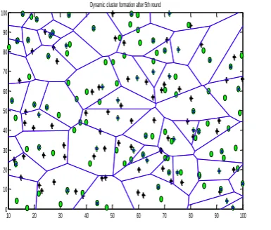
Dynamic cluster formation after 5th round
Fig.2 Dynamic Cluster formation for five rounds
Fig 2 shows the dynamic cluster formation during five rounds. Green circles (o) indicates normal nodes, plus sign (+) indicates advance nodes and circle with dot indicates the cluster head.
10 20 30 40 50 60 70 80 90 100 0
10 20 30 40 50 60 70 80 90 100
Dynamic cluster formation after 50th round
Cluster Heads Cluster Heads
Cluster Heads Cluster Heads
Fig.3 Dynamic Cluster formation for 50 rounds
In Fig.3 the dynamic cluster formation for fifty rounds is shown. Here yellow triangles indicate dead nodes. Dead nodes start occurring only after 20 rounds
10 20 30 40 50 60 70 80 90 100 0
10 20 30 40 50 60 70 80 90 100
Dynamic cluster formation after 100 rounds
Dead Nodes
Dead Nodes
Dead Nodes Dead Nodes
Fig.4 Dynamic Cluster formation for 100 rounds
In Fig.4 the dynamic cluster formation for hundred rounds is shown. Number of dead nodes are increased here. To reduce energy dissipation, each non-cluster head node uses power control to set the amount of transmit power based on the received signal strength of the cluster head. To reduce inter-cluster interference, each cluster in LEACH communicates using direct-sequence spread spectrum (DSSS). To reduce the possibility of interfering with nearby clusters and minimizes its own energy dissipation, each node adjusts its transmit power.
0 10 20 30 40 50 60 70 80 90 100 0.02
0.04 0.06 0.08 0.1 0.12 0.14 0.16
A
v
e
r
a
g
e
E
n
e
r
g
y
o
f
E
a
c
h
N
o
d
e
Number of Rounds Averege energy dissipated for 100 rounds
Fig.5 Average energy dissipated for 100 rounds
Average energy dissipated for 100 rounds is shown in Fig.5. Here it shows that as the number of rounds increases the average energy of each node is decree-sing. Nodes which have energy less than the average energy of all nodes will be dead.
Fig 6 shows that till 20 rounds no node is dead, for the
25th round 1 node is dead. From Fig 7 it is observed
0 5 10 15 20 25 0
0.1 0.2 0.3 0.4 0.5 0.6 0.7 0.8 0.9 1
X: 21 Y: 1
N
u
m
b
e
r
o
f
D
e
a
d
N
o
d
e
s
Number of Rounds
Fig.6 Number of dead nodes for 25 rounds
0 10 20 30 40 50 60 70 80 90 100 0
10 20 30 40 50 60 70 80 90
N
u
m
b
e
r
o
f
D
e
a
d
N
o
d
e
s
Number of Rounds
Fig.7 Number of dead nodes for 100 rounds
IV. CONCLUSION
In WSNs, clustering is important technique and selection of cluster head node is also important aspect. In this paper energy consumption is minimized by the cluster head during the process of extracting the essential data from the sensor nodes. Clustering has been used widely for efficient routing for the data communication from SNs to BS. Low Energy Adaptive Clustering Hierarchy (LEACH) protocol is the fundamental clustering based routing protocol for WSNs. Various parameters like cluster head formation, dissipated energies of each node, overall dead nodes are evaluated. It is observed clustering reduces the energy consumption and increase the life time of WSN. The parameters are selected based upon the applications and environment for which the WSN is operating.
REFERENCES
[1] Wendi B. Heinzelman, Anantha P. Chandrakasan, Senior and Hari Balakrishnan, An Application-Specific Protocol Archi-tecture for Wireless Microsensor Networks. IEEE Transactions on Wireless Communications 1(4): 660 - 670 (2002)
[2] Hai Lin, Lusheng Wang and Ruoshan Kong Energy Efficient Clustering Protocol for Large-Scale Sensor Networks. IEEE Sensors Journal 15(12): 7150 - 7160 (2015)
[3] S. Taruna, Sheena Kohli and G.N.Purohit, Distance Based Energy Efficient Selection of Nodes to Cluster Head in Homogeneous Wireless Sensor Networks. International Journal of Wireless & Mobile Networks 4(4):243-257 (2012)
[4] Arati Manjeshwar and Dharma P. Agrawal, TEEN: A Routing Protocol for Enhanced Efficiency in Wireless Sensor Networks. IEEE (2001)
[5] Kiran Maraiya, Kamal Kant and, Nitin Gupta, Efficient Cluster Head Selection Scheme for Data Aggregation in Wireless Sensor Network. International Journal of Computer Applications 23(9): (2011).
[6] Vinay Kumar Sanjeev Jain and Sudarshan Tiwari, IEEE Member Energy Efficient Clustering Algorithms in Wireless Sensor Networks: A Survey. International Journal of Computer Science 8(5): 259 - 268 (2011)
[7] Jin Wang, Xiaoqin Yang, Yuhui Zheng, Jianwei Zhang and Jeong-Uk Kim, An Energy-Efficient Multi-hop Hierarchical Routing Protocol for Wireless Sensor Networks. International Journal of Future Generation Communication and Networking 5(4): 89 (2012)
[8] Seema Yadav and Sanjiv Kumar Tomar, An Improved Clustering Approach in UWSN to improve Network Life. International Journal of Engineering Trends and Technology (IJETT) 4(5): 1826 - 1829 (2013)
[9] P. Agarwal and C. Procopiuc, Exact and approximation algorithms for clustering, Proc. 9th Annu. ACM-SIAM Symp. Discrete Algorithms, Baltimore, MD, Pp. 658–667 (1999). [10] J. Agre and L. Clare, An integrated architecture for cooperative
sensing networks. IEEE Computer 33: 106–108 (2000). [11] Deepika Gogia, Kamal Kumar Sharma and Deepak Kumar, A
Proposed Zonal Concept in LEACH Protocol for Wireless Sensor Network. International Journal of Research Aspects of Engineering and Management 1(2): 17-19 (2014).
[12] Rajni Rani and Gagan Kumar, A Noval Minimum Transmission LEACH Protocol for WSN (Proposed) IJSRD - International Journal for Scientific Research & Development 3(6): 28-30 (2015)
[13] Nitin Mittal, Davinder Pal Singh, Amanjeet Panghal and R.S. Chauhan, Improved LEACH Communication Protocol for WSN NCCI 2010 -National Conference on Computational Instrumentation CSIO Chandigarh, INDIA, 19-20 March (2010) [14] Shreesha Bhat, Vasudeva Pai, Pranesh and V Kallapur, Energy Efficient Clustering Routing Protocol based on LEACH for WSN. International Journal of Computer Applications 120(13): 17 - 20 (2015)
[15] Lalita Yadav and Ch. Sunitha, Low Energy Adaptive Clustering Hierarchy in Wireless Sensor Network (LEACH). International Journal of Computer Science and Information Technologies, 5 (3): 4661-4664 (2014)
[16] W. Heinzelman, A. Chandrakasan, and H. Balakrishnan, Energy-efficient routing protocols for wireless microsensor networks, Proc. 33rd Hawaii Int. Conf. System Sciences (HICSS), Maui, HI, Jan. (2000).
[17] A. Chandrakasan, R. Amirtharajah, S.-H. Cho, J. Goodman, G. Konduri, J. Kulik, W. Rabiner, and A. Wang, Design considerations for distributed microsensor systems, Proc. IEEE Custom Integrated Circuits Conf. (CICC), San Diego, CA, Pp. 279–286 (1999).
[18] M. Dong, K. Yung, and W. Kaiser, Low power signal processing architectures for network microsensors, Proc. Int. Symp. Low Power Electronics and Design, Monterey, CA, Pp. 173–177 (1997).
[19] P. Agarwal and C. Procopiuc, Exact and approximation algorithms for clustering, Proc. 9th Annu. ACM-SIAM Symp. Discrete Algorithms, Baltimore, MD, Pp. 658–667 (1999) Fengjun Shang, Yang Lei An Energy-Balanced Clustering Routing Algorithm for Wireless Sensor Network Wireless Sensor Network 2: 777-783 (2010)
[20] Nilu Kumari, D.K. Gupta and Manoj Kumar Sah, Improved TEEN Routing Protocol with Multi Hop and Multi Path in Wireless Sensor Networks International Journal of Computer Applications 129(7): 11- 16 (2015).