_____________________________________________________________________________________________________ *Corresponding author: E-mail: iamtcd1993@163.com;
Environmental Kuznets Curve of Household
Electricity Consumption in China: Based on Spatial
Econometric Model
Caidan Tan
1*1Nanjing University of Aeronautics and Astronautics, China.
Author’s contribution
The sole author designed, analysed, interpreted and prepared the manuscript.
Article Information
DOI: 10.9734/JENRR/2019/v2i330080 Editor(s): (1)Dr. Fernando de Lima Caneppele, Professor, Departamento de Engenharia de Biossistemas, University of Sao Paulo, Brazil. (2)Dr. Salisu Muhammad Lawan, Department of Electrical and Electronics Engineering, Kano University of Science and Technology (KUST) Wudil, Nigeria. Reviewers: (1) Lifeng Wu, Hebei University of Engineering, China. (2)Soava Georgeta, University of Craiova, Romania. Complete Peer review History:http://www.sdiarticle3.com/review-history/48161
Received 10 January 2019 Accepted 24 March 2019 Published 30 March 2019
ABSTRACT
In this paper, the spatial measurement model is introduced into the environmental Kuznets curve to investigate the impact of income on household electric carbon emissions. The spatial correlation diagnosis was made by using Moran scatterplot and Moran index. The results of spatial error model show that the environmental Kuznets curve of household electric carbon emissions is inverted N-shaped carve. The maximum and minimum values of environmental Kuznets curve are per capita real GDP of RMB 10198 Yuan and RMB 44355 Yuan (at constant price in 2005). It means that the per capita household electric carbon emissions are still on the rise in most provinces of China.
Keywords: Household electric carbon emission; environmental Kuznets curve; spatial measurement model.
1. INTRODUCTION
The entry into force of the Kyoto protocol in 2005, the Copenhagen climate conference in 2009 and the formulation of the Paris agreement in 2016
revealed that all countries in the world have paid great attention to the issue of climate change [1-3]. At present, greenhouse gases, such as carbon dioxide, is a key factor leading to climate change. Energy conservation and emission
reduction is an urgent need to cope with global climate change and an inevitable choice to build a resource-conserving and environment-friendly society.
Along with the economic growth and the improvement of residents' living standards, the household electricity consumption continues to grow rapidly, accounting for an increasing proportion of the electricity consumption of the whole society. According to the data of electricity consumption [4], electricity consumption reached 5919.8 billion kWh, up by 5.0% year on year; Urban and rural residents consumed electricity of 805.4 billion kWh, up 10.8% year on year. The proportion of household electricity consumption on the total electricity consumption is only slightly more than 13%, while that of developed countries is about 20%. At the same time, through the horizontal comparison of the data of per capita household electricity consumption in various countries in 2015, the per capita household electricity consumption in most developed countries is 1000~4000 kWh, and the per capita household electricity consumption in the United States and Canada has reached 4486 kWh and 4617 kWh respectively. However, China's per capita household electricity consumption is 529 kWh, which is about 1/9 that of the United States and Canada and far lower than the level of developed countries. Through the lateral comparison of the data of per capita household electricity consumption in various provinces of China in 2015, Fujian ranked first with per capita household electricity consumption of 898.57 kWh; per capita household electricity consumption of other developed provinces and cities is more than 700 kWh, such as Beijing, Shanghai, Zhejiang and Guangdong; that is relatively low in most of the less developed provinces (such as Xinjiang, Qinghai, Ningxia and Gansu), which is under 400 kWh; that is 400~700 kWh basically in other provinces. That means there is still huge room for growth. So household electricity carbon emissions cannot be ignored in order to reduce carbon emissions.
Income is one of the main driving factors of household electricity consumption, and the difference in household electricity consumption between different regions can be explained by the income gap between China and developed countries or among 30 provinces. Countries or regions with higher economic development tend to have higher per capita household electricity consumption. For developed economies, the per capita energy consumption basically shows an
inverted u-shaped pattern [5]. Given the trend of increasing income, will per capita household electricity carbon emissions continue to grow in China or will they start to decline when the income reaches a certain level? If there is a turning point, where is the turning point? In order to answer these questions, the current general method is the empirical research of the environmental Kuznets curve (EKC) to judge whether and when the pollution peak exists. It is helpful for the government to make more reasonable policies on energy conservation and emission reduction to understand the current situation of carbon emission from household electricity in China.
2. LITERATURE REVIEW
EKC theory originated from the study on the relationship between atmospheric environment and per capita income in North American Free Trade Agreement (NAFTA) [6]. This study found that there was a significant inverted U-shaped curve relationship between smog, suspended matter and per capita income. Later, Panayotou [7] studied the relationship between different environmental pollutants and income levels based on Grossman and Krueger’s study, and found that there was also an inverted U-shaped curve relationship between the two, which was called the environmental Kuznets curve (EKC). EKC theory is an empirical hypothesis, and the related researches mainly focus on the empirical aspects. EKC theory assumes that environmental quality will deteriorate with income growth, but environmental quality will improve with income growth when income reaches a certain level. In essence, the EKC theory reflects the process of transforming the economic development model with high energy consumption and high pollution into a resource-conserving and environment-friendly one, indicating that the economic growth target is beneficial in the long run.
emissions of a certain industry or department in a certain region. For example, Yan et al. [9] found an inverted N-shaped curve relationship between the carbon emissions of the construction industry in Guangdong province and the per capita output value of the construction industry based on the EKC. Tian and Xie [10] found that China's agricultural per capita carbon dioxide emissions and per capita GNP showed an inverted U-shaped curve relationship based on the research of EKC theory, and China's agricultural carbon emissions were at the left of the inflection point of the inverted U-shaped curve. Current form of EKC not only limited to the inverted U-shaped curve because the Non-income factors can also affect the form. The third power of item of the per capita GDP is used when verifying the existence of EKC. Because the measure of the inflection points of the corresponding high per capita income levels when only contains second power of per capita GDP [11]. And the non-income factors should be considered too.
In recent years, there are more and more researches on the combination of EKC and spatial econometric model. Yang et al. [12] studied the relationship between air quality and economic growth of 46 cities in China by combining EKC and spatial econometric model. Wu and Tian [13] analyzed the spatial correlation, EKC shape and determinants of provincial environmental pollution based on the EKC theory and spatial econometric model. Hao et al. [14] found that there is strong spatial correlation between China's economic growth and energy or electricity consumption per capita, and the energy or power consumption per capita and Per capita GDP have the N-shaped EKC relationship by choosing the appropriate spatial econometrics model to the Chinese provincial per capita energy consumption and power consumption per capita for empirical research.
When investigating the relationship between household electricity carbon emission and income, it is unreasonable to use EKC equation directly, because the hypothesis of spatial data independence of EKC is obviously inconsistent with reality. First of all, China's regional economic development is unbalanced. Each region has its own characteristics and forms its own "convergence club". Second, the economic behavior of the current decision of regional economies is often affected by the previous or current behavior of other economies [15], for example local government perhaps reference the policies of electricity price and energy
conservation of the neighborhoods and then make the relevant policies. And city is a nodes of social economic and social resources in the economic region and the residents' consumption behavior is related to economic and social development level [16]. Moreover, there are differences in the endowment of power resources between different provinces in China, and there are contradictions between the endowment of power resources and demand, which leads to a large number of power transmission and allocation among regional power grids in China. However, the carbon emission coefficient of power in different regions is obviously different. So it is unreasonable to investigate the influence of local electricity carbon emissions on local regions only from the perspective of consumption [17]. Finally, temperature will also affect the electricity consumption of residents. Chen et al. [18] found that the colder the household area is, the less willing residents are to save energy, and the temperature of adjacent areas is often similar. Therefore, it may be biased to ignore the spatial characteristics when examining the household electricity carbon emissions. Spatial econometrics abandons the traditional assumption that econometrics has no spatial relevance, and introduces a spatial weight matrix to consider the impact of spatial correlation on economic activities, so as to eliminate the spatial bias in the calculation results.
that population density may affect the intensity of household carbon emission by influencing the size of houses. Ding [21] and Wang et al. [22] decomposed the carbon dioxide emissions of household energy consumption and found that the population scale effect, income level, urban-rural structure and other factors are the key factors affecting the carbon emissions of household energy consumption.
Therefore, this chapter will introduce urbanization rate and population density to expansion EKC theory and select the space panel econometric model to study the household electricity carbon emissions in China. The main innovation of this paper is to investigate the spatial correlation of household electric carbon emissions. The rest of this paper is structured as follows: the third part briefly introduces the model, estimation method and data to be used in this paper; the fourth part carries on the spatial autocorrelation test, and uses the spatial econometric model to carry on the demonstration analysis; the fifth part is the conclusion.
3. ECONOMETRIC MODEL
3.1 Basic Econometric Model
3.1.1 Model reference form
This paper introduces the EKC equation containing the third power terms of per capita real GDP as the basic form of the regression equation, and introduces the controlling variables, urbanization rate and population density, to expand the EKC equation:
lnE, =α + lny, + lny, + lny, +
lnUR, + lnPD, +φ, (1)
Ei,t represents carbon emission generated by per capita household electricity consumption of the province i in the year t, yi,t represents per capita real GDP of the province i in the year t, Although per capita disposable income is often used to investigate the impact on household electricity consumption, per capita GDP is also used in some studies [23]. URi,t and PDi,t represent two control variables: urbanization rate and population density. αi is a random perturbation term, and φi,t is a random perturbation term. Different values of β1, β2 and β3 will lead to different shapes of curves, which can be divided into the following 7 cases:
(1) When β1=β2=β3=0, there is no relationship between per capita household electricity carbon emissions and per capita GDP;
(2) When β1<0 and β2=β3=0, per capita household electricity carbon emissions decrease with the increase of per capita GDP;
(3) When β1>0 and β2=β3=0, per capita household electricity carbon emissions increase with the increase of per capita GDP;
(4) When β1<0, β2>0 and β3=0, there is a U-shaped relationship between per capita household electricity carbon emissions and per capita GDP;
(5) When β1>0, β2<0 and β3=0, there is an inverted U-shaped relationship between per capita household electricity carbon emissions and per capita GDP. When carbon emissions start to decline, the
turning point is
1 2
2
t
y e
;
(6) When β1<0, β2>0 and β3<0, there is an inverted N-shaped relationship between per capita household electricity carbon emissions and per capita GDP, which means that per capita household electricity carbon emissions start to increase at the first turning point, and decrease with the growth of per capita GDP at the second turning point.
(7) When β1>0, β2<0 and β3>0, there is a N-shaped relationship between per capita household electricity carbon emissions and per capita GDP, which means that the per capita household electricity carbon emissions start to decrease at the first turning point, and increase with the growth of per capita GDP at the second turning point.
3.1.2 Spatial econometric model
Before introducing spatial autocorrelation factors, spatial correlation test of data should be carried out first. The spatial correlation index is Moran index [24], and its calculation formula is:
I = ∑∑ ∑∑ ,( ̅)( ̅)
, ∑ ( ̅) =
∑ ∑ ,( ̅)( ̅)
∑ ∑ ,
(2)
Where, I is the Moran index, xi is the observed value of the explained variables in the region i, n
otherwise,Wi,j=0. The value range of Moran index is [-1, 1]. When Moran index is greater than 0, it means there is positive spatial autocorrelation; when it is less than 0, it means there is negative spatial correlation.
When Moran index indicates the spatial dependence of panel data, the spatial panel model can be introduced, which may contain the dependent variable of spatial lag or the error term of spatial autoregressive. Elhorst [25] proposed three basic spatial econometric models, namely spatial lag model (SLM), spatial error model (SEM) and spatial Durbin model (SDM).
The basic form of SLM is:
Y, =ρ∑ , , + + , + +η +φ, (3)
Where, i=1,…,N, and t=1,…,T. Yi,t represents the cross-sectional observation value of unit i at time t, which is an N×1 dimensional vector composed of explained variables. Xi,t is the explanatory variable. Ρ represents the spatial regression coefficient, Wi,j represents the space weight matrix, the paper uses the adjacent weight matrix, namely, such as space region i
and j adjacent, then Wi,j=1, otherwise Wi,j=0. α denotes the constant term, β denotes the estimated coefficient of the explanatory variable; μi stands for space effect; ηt means time fixed effect; φi,t means independent homodistributed error term.
The basic form of SEM is:
Y, =βX, +μ +η +φ, (4)
φ, =λ∑ , , + , (5)
Where, φi,t is the spatial autocorrelation error term, λ is the spatial error coefficient.
The basic form of SDM is:
Y, =ρ∑ , , + , + ∑ , , + +η +
φ, (6)
3.1.3 Correlation testing and estimation methods
This article is based on the steps adopted by Elhorst [25]. Firstly, estimate the spatial panel data model. The estimation methods respectively
are mixed OLS, space-fixed effect, time-fixed effect and time-fixed and space-fixed effect. The likelihood ratio test is applied to the fixed effects, and whether the spatial panel data overlooked the space effect of panel data is tested according to each kind of model of LM statistics, which is used to determine what kind of spatial econometrics model.
Secondly, Wald test and LR test are used to test whether SDM can be simplified into SLM or SEM. If both null hypotheses are rejected, the SDM provides the best fit. Finally, Hausman test is used to select random effects and fixed effects.
3.2 Data Description
This paper mainly adopts two kinds of index data. One is the per capita real GDP used to reflect the level of regional economic development, which is expressed by yi,t. The other is the carbon emissions caused by the per capita household electricity consumption of provincial residents over the years, which is used to reflect the living electricity consumption of residents, represented by Ei,t. In the study, the per capita value of household electricity carbon emissions can eliminate the scale effect. Referring to other EKC empirical studies, this paper selected population density and urbanization rate as control variables. The electricity consumption data used in this study were derived from China Energy Statistics Yearbook from 2006 to 2016, and the data of 30 provinces, municipalities and autonomous regions (except Tibet, Hong Kong, Macao and Taiwan) were selected.
According to Table 1, the per capita household electricity carbon emissions of residents in each province are calculated as follows:
E, = CE, ∗ ,
, (7)
Where, Ei,t represents the per capita household electricity carbon emissions of residents in the province i in the year t(i =1,2... , 30; t = 1, 2,... , 11), and the unit is kg/ person; CEi,t represents the household electricity consumption in the province i in the year t, and the unit is kWh; Fi.k represents the grid emission factor of the region of province i, and the unit is kgCO2/kWh; ni,t refers to the resident population of the province i
Table 1. Carbon emission factors of regional power grid in 2015
Region Grid carbon emission factor (unit: kgCO2/kWh) North China 1.0416
Northeast China 1.1291 East China 0.8112 central China 0.9515 Northwest China 0.9457 South China 0.8959
Note: the carbon emission factor of China's regional power grid in 2015 is the weighted average of the marginal power emission factor from 2011 to 2013
Table 2. Descriptive statistical results of variables
Variable name Unit Mean Standard
deviation
Maximum Median Minimum
Per Capita Household Electricity Carbon Emissions
kg/person 357.75 153.11 838.65 339.35 118.90
Per Capita Real GDP
Yuan(in the constant of 2005)
28735.49 17674.55 95560.13 24012.71 5376.46
Urbanization Rate
% 51.74 14.13 89.60 49.22 26.87
Population Density
persons/square kilometer
436.96 632.75 3772.94 279.39 7.54
4. EMPIRICAL RESULTS AND ANALYSIS
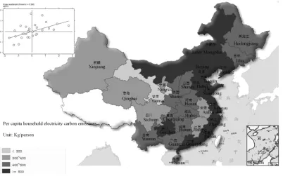
4.1 Per Capita Household Electricity Carbon Emissions Distribution and Spatial Autocorrelation Analysis
The software STATA was used to draw the distribution map and Moran scatter plot of the per capita household electricity carbon emissions of Chinese residents in 2005, 2010 and 2015 (seen in Fig. 1, Fig. 2 and Fig. 3). When drawing the carbon emissions distribution map, the same segmentation method is used: 0~300, 300~400, 400~500 and above, and the unit is kg/person. Though the distribution maps of three years, it can be found that the level of per capita household electricity carbon emissions is similar in the adjacent areas. At the same time, per capita household electricity carbon emissions are gradually increased, and that of the coastal areas grow faster. The provinces above 500kg/person carbon emissions are mainly concentrated in coastal areas. It can be concluded from the Moran scatter diagrams that the global Moran’s I of per capita household electricity carbon emissions is greater than zero, and the significance test of 1% indicates that per capita household electricity carbon emissions have a significant spatial positive correlation (distribution
Fig. 1. The distribution map and Moran scatter plot of per capita household electricity carbon emissions of Chinese residents in 30 province in 2005
Fig. 3. The distribution map and Moran scatter plot of per capita household electricity carbon emissions of Chinese residents in 30 province in 2015
4.2 Spatial Diagnostic Test
To test which model could better fit the data, the non-spatial panel data model was first analyzed, and the classical Lagrange Multiplier Statistic (LM-lag, LM-error) and Robust Lagrange Multiplier Statistic (Robust lag, Robust LM-error) were used to select the spatial panel econometric model [15]. The equation (1) was estimated by mixed OLS, space-fixed effect, time-fixed effect and space-fixed and time-fixed effect.
Due to the different situation of each province and city, there may be omission variables that do not change with time. The fixed effect is still the first choice for two reasons according to the current empirical analysis. This is because: Firstly, when modeling spatial panel data, the fixed effect is usually more appropriate than the random effect. Secondly, Lee and Yu [26] believed that the fixed effect was robust, and the calculation was as simple as the random effect model. Therefore, the fixed effect model is considered in this paper. The estimated results are shown in Table 3.
The estimation results of the non-spatial panel data model show that the estimation results of
the time-fixed effect model are the best in the set of estimation methods. Since the estimators of independent variables and control variables of the time-fixed effect model are both significant at the significance level of 1%, the model fitting degree reaches 0.777, and the D-W statistic close to 2 indicates that the sequence correlation problem is not significant. Due to the introduction of the cubic form of regional per capita GDP in explanatory variables, the EKC curve estimated by the time-fixed effect model is of inverted N-shaped, and there are EKC minimum point and maximum point. The EKC minimum point corresponds to a per capita GDP of 5,014 Yuan (at constant price in 2005), while the EKC maximum point corresponds to a per capita GDP of 67,507 Yuan. The LM-lag and LM-error test results of the time-fixed effect model showed that the time-fixed effect model rejected the hypothesis that there was no spatial error term at the significance level of 1%, and whether there was a spatial lag term did not pass the test. Therefore, the spatial error model of time fixed effect was used for estimation next (seen in Table 4).
0.875, which was higher than that of the non-spatial and time-fixed effect model, indicating that the spatial error model could better fit the data. The spatial error coefficient is 0.302 at the significance level of 1%, which again indicates that the household electricity carbon emissions have a strong spatial autocorrelation. At the significance level of 1%, the logarithmic coefficients of per capita GDP are all significant, and the coefficients of the primary, secondary and tertiary terms are negative, positive and
negative respectively, indicating that the environmental Kuznets curve of household electricity carbon emissions is of inverted N-shaped. The per capita real GDP of the maximum point and minimum point of EKC are 10198 Yuan and 44355 Yuan (at constant price in 2005) respectively. That means when per capita real GDP of the region is less than 10198 Yuan, per capita household electricity carbon emissions of residents are in a state of decline. When per capita real GDP of the region is
Table 3. Estimation results of non-spatial panel model
Estimation method Mixed OLS Space-fixed Time-fixed Time-fixed and space-fixed
C 130.911**
(3.604)
Lny -39.806***
(-3.677)
-5.310 (-0.974)
-52.386*** (-5.599)
-6.918 (-1.361)
(lny) 2 4.125***
(3.847)
0.663 (1.216)
5.283*** (5.710)
0.722 (1.424)
(lny) 3 -0.140***
(-3.949)
-0.024 (-1.344)
-0.176*** (-5.785)
-0.025 (-1.487)
lnUR -0.052
(-0.505)
1.060 *** (6.710)
0.596*** (5.686)
1.232*** (7.805)
lnPD 0.033***
(3.349)
0.1496 (0.906)
0.0523*** (6.057)
-0.752 (-3.733)
R2 0.821 0.934 0.777 0.513
σ2 0.036 0.006 0.026 0.005
D-W 1.620 1.873 2.132 2.003
Log-likelihood 82.318 370.039 136.258 396.110 LM spatial lag 59.453***
(p=0.000)
9.790*** (p=0.002)
0.298 (p=0.585)
0.467 (p=0.495) Robust LM spatial lag 15.528***
(p=0.000)
0.139 (p=0.710)
5.919** (p=0.015)
10.776*** (p=0.001) LM spatial error 59.857***
(p=0.000)
19.812*** (p=0.000)
13.001*** (p=0.000)
1.971 (p=0.160) Robust LM spatial error 15.932***
(p=0.000)
10.160*** (p=0.001)
18.622*** (p=0.000)
12.280*** (p= 0.000) per capita real GDP (Yuan)
corresponding to the EKC minimum point
8604 —— 5014 ——
Real Per capita GDP (Yuan) corresponding to EKC maximum point
56954 —— 67507 ——
Note: lny represents the logarithm of carbon emissions generated by per capita household electricity consumption at the provincial level, lny represents the logarithm of per capita income at the provincial level, lnUR represents the logarithm of urbanization rate, lnPD represents the logarithm of population density at the provincial
level, lnL represents the logarithm of maximum likelihood value, and D-W represents the statistic of Durbin-Waston. The estimated value of the explanatory variable is the corresponding t value in square brackets, and the
Table 4. Estimation results of spatial error model
Explanatory variables Space error model of
time - fixed effect
lny -56.291*** (-5.951)
(lny) 2 5.684*** (6.073)
(lny) 3 -0.190*** (-6.151)
lnUR 0.529*** (5.116)
lnPD 0.051*** (5.219)
λ 0.302*** (4.576)
σ2 0.025
R2 0.8705
corr-R2 0.7765
log-likelihood 143.723
The per capita real GDP (Yuan) corresponding to the EKC minimum point
10198
Real Per capita GDP (Yuan) corresponding to the EKC maximum point 44355
between 10198 and 44355 Yuan, per capita household electricity carbon emissions are on the rise. When per capita real GDP of the region is greater than 44355 Yuan, per capita household carbon emissions are in a state of decline. In 2015, the per capita real GDP (at constant price in 2005) of 20 provinces was between 10198 and 44355 Yuan, and per capita real GDP (at constant price in 2005) of 10 provinces was above 44355 Yuan. Per capita household electricity carbon emissions are still rising in most of the provinces in China. Income is a key variable affecting residents' electricity consumption, and its influence on residents' electricity demand is mainly through the following two ways: first, indirectly affecting residents' electricity consumption by affecting their electric complementary-home appliances; second, through the impact of residents on the frequency of electrical appliances to produce a direct impact. At the same time, the coefficient of urbanization rate and population density is also significantly positive, indicating that the carbon emissions of household electricity will also increase with the acceleration of urbanization process and the increase of population. In the context of economic growth, accelerated urbanization and increasing population, reducing household carbon emissions from electricity can improve energy conservation and emission reduction.
5. CONCLUSION
This paper selects the panel data of 30 provinces in China from 2005 to 2015, and calculates the
urbanization process, reducing household carbon emissions is still the key to energy conservation and emission reduction.
COMPETING INTERESTS
Author has declared that no competing interests exist.
REFERENCES
1. Grubb M, Vrolijk C, Brack D. Kyoto protocol: A guide and assessment. Molecular Ecology. 1999;3(8):2121-33. 2. Bodansky D. The copenhagen climate
change conference-A post-mortem. The American Journal of International Law. 2010;104(2):230-240.
3. Falkner R. The paris agreement and the new logic of international climate politics. International Affairs. 2016;92(5):1107-1125. 4. National Bureau of Statistics of the People’s Republic of China. China Energy Statistics Yearbook; 2016.
5. Zheng Xin-ye. A research report on household energy consumption in China. Science Press, 2016;130-131.
6. Grossman GM, Krueger AB. Environmental impacts of a North American free trade agreement. Social Science Electronic Publishing. 1991;8(2):223-250.
7. Panayotou T. Empirical tests and policy analysis of environmental degradation at different stages of economic development. IIo Working Papers. 1993;4.
8. Hu Chu-Zhi, Huang Xian-Jin, Zhong Tai-Yang, et al. Character of Carbon emission in China and its dynamic development analysis. China Population Resources and Environment. 2008;03:38-42.
9. Yan Wei-Qian, She Li-Zhong, Zhong Shi-Yu, et al. Empirical analysis on construction industry of carbon emission Kuznets curve in Guangdong province. Journal of Civil Engineering and Management. 2018;35(02):189-194. 10. Tian Wei, Xie Dan. Agricultural
environmental kuznets curve’s test and analysis in China: Based on the view of carbon emission [J].Ecological economy. 2017;33(02):37-40.
11. Xu Guang-Yue, Song De-Yong. An empirical study of the environmental Kuznets curve for china’s carbon emissions——Based on provincial panel data [J]. China Industrial Economics. 2010;05:37-47.
12. Yang Hai-Sheng, Zhou Yong-Zhang, Wang Xi-Z. Spatial metrological test of environment Kuznets curve of China’s urban. Statistics and Decision. 2008;10:43-46.
13. Wu Yu-Ming, Tian Bin. The extension of regional environmental Kuznets curve and its determinants: An empirical research based on spatial econometrics model [J]. Geographical Research. 2012;31(04):627-640.
14. Hao Yu, Liao Hua,Wei Yi-Ming. The environmental Kuznets curve for China's per capita energy consumption and electricity consumption: An empirical estimation on the basis of spatial econometric analysis. China Soft Science. 2014;01:134-147.
15. Le Sage JP, Pace RK. Introduction to spatial econometrics. Boca Raton, US: CRC Press Taylor and Francis Group. 2009;513-514.
16. Mi Ling-Yun. Research on urban residents low carbonization energy consumption behavior and policy guidance. China University Mining and Technology; 2011.
17. Fu Kun, Qi Shao-Zhou. Accounting method and its application of provincial electricity CO2 emissions responsibility. China Population Resources and Environment. 2014;24(04):27-34.
18. Chen CF, Xu X, Day JK. Thermal comfort or money saving? Exploring intentions to conserve energy among low-income households in the United States. Energy Research & Social Science. 2017;26:61-71. 19. Lin Bo-Qiang, Liu Chang. Impacts of
income and urbanization on urban home appliance consumption. Economic Research Journal. 2016;51(10):69-81,154. 20. Jones C, Kammen DM. Spatial distribution
of US household carbon footprints reveals suburbanization undermines greenhouse gas benefits of urban population density. Environmental Science & Technology. 2014;48(2):895-902.
21. Ding Yong-Xia. Study on temporal-spatial variation of household energy consumption in China. Lanzhou University. 2011;28- 31.
23. Sun Y, Yu Y. Revisiting the household electricity demand in the United States: A dynamic partial adjustment modelling approach. Social Science Journal. 2017;54(3).
24. Moran P. A test for serial correlation of residuals. Biometrika. 1950;37:178-181.
25. Elhorst JP. Matlab software for spatial panels. Inter-national Regional Review. 2012;1-17.
26. Lee LF, Yu J. Estimation of spatial autoregressive panel data models with fixed effects. Journal of Econometrics. 2010;154(2):165-185.
_________________________________________________________________________________ © 2019 Tan; This is an Open Access article distributed under the terms of the Creative Commons Attribution License
(http://creativecommons.org/licenses/by/4.0), which permits unrestricted use, distribution, and reproduction in any medium,
provided the original work is properly cited.
Peer-review history: