ORIGINAL ARTICLE
Jung-Kwon Oh · Kugbo Shim · Kwang-Mo Kim · Jun-Jae Lee
Quantifi cation of knots in dimension lumber using a single-pass
X-ray radiation
Abstract The knot depth ratio (KDR) evaluation method was designed to quantitatively evaluate the amount of knot in dimension lumber by a single-pass X-ray radiation. To verify the proposed method, KDR values for 38-mm-thick specimens were predicted, and they were compared with the actual measured KDR values. The knot is surrounded by the transition zone, and the density of the knot and the transition zone is higher than the clear wood. Because the average density of the transition zone was similar to the knot density, it was found that the proposed method gives the KDR values for the knot area including the transition zone. The coeffi cients of determination between the pre-dicted and measured KDR values were 0.87 and 0.83 for Japanese larch and red pine specimens, respectively. Using the KDR information, the ratio of knot area including tran-sition zone to cross-sectional area was calculated. The pres-ence of latewood and earlywood in the same path of the X-ray radiation caused discrepancies in the estimation of KDR values because the density of latewood is much higher than that of earlywood. Fortunately, latewood and early-wood are repeated in a cross section, so the amount of overestimation and underestimation was expected to be nearly identical. As expected, the relationship between the predicted area ratio and the real area ratio of knot and transition zone was strong with R2
values of 0.89 and 0.93 for Japanese larch and red pine specimens, respectively.
Key words Knot · Knot depth ratio · X-ray · Defect · Image analysis
K. Shim · K.-M. Kim
Department of Forest Products, Korea Forest Research Institute, Seoul 130-712, Republic of Korea
J.-K. Oh · J.-J. Lee (*)
Research Institute for Agriculture and Life Sciences, Department of Forest Sciences, Seoul National University, San 56-1 Sillim 9 dong Gwanak-gu, Seoul 151-921, Republic of Korea
Tel. +82-28-80-4782; Fax +82-28-71-0156 e-mail: [email protected]
Introduction
Knots are almost always present in lumber and are known to be the most serious defect, because they greatly reduce the strength of lumber and the quality of products. There-fore, nondestructive evaluation of knots is crucial for esti-mation of lumber strength and yield of wood.
Riberholt and Madsen1
reported that the failure of lumber is primarily initiated at the weakest cross section that corresponds to the largest knot or a group of knots. In the destructive bending test, failure is almost exclusively caused by knots. Schniewind and Lyon2
tested redwood timber and in 95% of the cases, failure occurred at knots or local slope of the grain, which was mostly related to the knots. In a study by Johansson et al.,3
91% of failures were caused by knots.
In order to evaluate knots, there are various nondestruc-tive evaluation methods such as acousto-ultrasonic4
and microwave scanning,5
stress wave propagation,6
and image processing using optical instruments.7
However, these studies focused only on detection of knots.
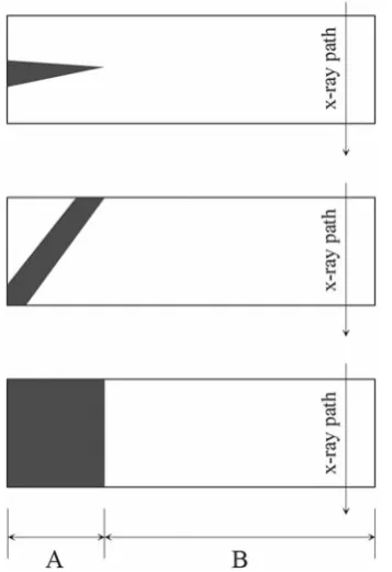
In general, the knot is regarded as a loss of cross section. Because knots are less resistant to stress than clear wood, the strength of lumber is inversely proportional to the knot area ratio (KAR), which is defi ned as the ratio of knot area to the cross-sectional area.2
For instance, there are three shapes of knot as shown in Fig. 1. Among the three lumbers, the lumber containing the largest knot area (bottom in Fig. 1) was expected to be the weakest. However, most current nondestructive methods can determine the presence of knots and cannot quantify the amount of knots in the lumber thickness. Consequently, these knots cannot be distinguished from each other and may be regarded as the same size. However, because the KARs are different from each other, these lumbers show different strengths.
Schniewind and Lyon2
estimated the KAR using the knot information observed on the surface of the lumber. The value of the KAR was correlated with the strength of the lumber. The current visual grading rules are also based on the KAR concept, such as Standard Grading Rules for
The amount of absorbed energy depends on the density of the section of wood through which the X-ray passed. This density can be calculated using the attenuation equation of Beer’s Law and X-ray radiography.10,11
It is well known that the density of knots is twice that of normal wood.12
The
Materials and methods
Measurement of knot density
Knot density was measured by converting the X-ray image of a 10-mm-thick specimen into density. To verify density measurement using X-ray radiation, 19 wood specimens (10 mm thickness) were prepared. To provide a large variation in density, some samples contained knots and juvenile wood, and various wood species of Japanese larch (Larix kaempferi), Japanese cedar (Cryptomeria japonica), and red pine (Pinus densifl ora) were used (Table 1). Because X-ray attenuation depends on the thickness of the specimen, the use of different thicknesses is required to verify the method. Twenty-four 38-mm-thick specimens were also prepared (Table 1).
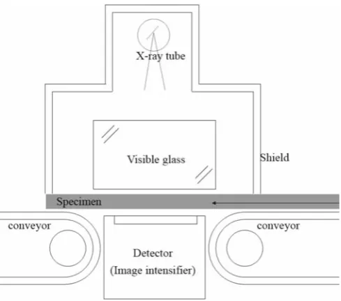
X-ray scanning equipment consisted of an X-ray tube, a shield to protect the inspector, and an X-ray detector (Figs. 2 and 3). A Thales image intensifi er (TH9429) was used as the X-ray detector. This detector can produce an X-ray digital image immediately, and no developing or printing is required. The resolution of the X-ray images was 2.7 dots per millimeter. The densities of specimens were calculated using Beer’s Law (Eq. 1).10,11
The intensity of X-ray radiation was quantifi ed using a surveymeter (RSM-300, Iljin Radiation Engineering). The mass attenuation coeffi cient was experimentally determined for each thickness of the specimen. In order to compare the density predicted by X-ray scanning with the real density, the air-dry densities of the same specimens were measured according to Eq. 2.
ρ μ
= 1⎛⎝ ⎛⎝ 0⎞⎠⎞⎠
t I
I
log (1)
Fig. 1. Cross-sectional view of an example for the different knot
shapes. A, The zone identifi ed as a knot by knot detection; B, the zone identifi ed as a clear part by knot detection
Table 1. Specimens used to verify density measurement by X-ray radiation
Thickness of specimen (mm)
Species Total number of specimens
Number of specimens with knots
Number of specimens with pith
10 Japanese larch 7 2 1
Japanese cedar 5 3 2
Red pine 7 1 1
38 Japanese larch 7 1 1
Japanese cedar 8 2 2
where r is the density evaluated by X-ray radiation (g/cm3
); m is the mass attenuation coeffi cient (cm2
/g); t is thickness of the specimen (cm); I0 is the intensity of incident radiation
(Sv/h); I is the intensity of transmitted radiation (Sv/h).
D W V
= air-dry
air-dry
(2)
where D is the air-dry density (g/cm3
); Wair-dry is the weight
of the specimen (g); Vair-dry is the volume of the specimen
(cm3).
To measure the knot density, 54 knots of Japanese larch and 42 red pine knots of 10 mm in thickness were prepared. All specimens were prepared to have the knot penetrate the specimen thickness (10 mm) at a right angle (Fig. 4).
Specimens were set to allow X-rays to pass through the 10-mm thickness of the specimens. The X-ray images were converted into density by using Beer’s Law (Eq. 1).10,11
In
this study, the wide face of each specimen was divided into three zones: knot zone, transition zone, and clear part zone. The transition zone was defi ned as the area between the knot zone and the clear part zone. At fi rst, the clearly identifi ed knot zone and clear part were separated from other zones. All area not classifi ed as clear part or knot zone was classifi ed as transition zone. Some obscure areas were identifi ed by observing the wide face of the specimen using a magnifying camera (ICSL-305, Sometech). The density of each zone was obtained by extracting the partial image for each zone from the raw X-ray image and converting the partial image into density by Beer’s Law.
Verifi cation of knot depth ratio prediction
Method to predict knot depth ratio
In Korea, Japanese larch and red pine are most frequently used for structural purposes. Therefore, 35 pieces of Japanese larch and 43 pieces of red pine were sampled from commercial mills. The size of each specimen was 38 × 140
× 3600 mm and the specimens were kiln-dried to an average moisture content of approximately 18%.
X-ray images were taken at cross sections containing knots. Specimens were set to allow X-rays to pass through the 38-mm thickness of the specimen. Eighty-fi ve knots of Japanese larch and 73 knots of red pine were investigated. Using a knot detection algorithm,13
two sheets of X-ray images were prepared for each specimen: knot X-ray image and clear part X-ray image.
The knot depth ratio (KDR) was defi ned as the ratio of knot thickness (tknot) to lumber thickness (t) (Fig. 5,
Eq. 3).
KDR=tknot
t (3)
Even though the densities of clear wood and knots vary over a wide range, it was assumed that the densities of both Fig. 2. Photograph of X-ray equipment
Fig. 3. Schematic drawing of X-ray test equipment
Fig. 4a, b. Specimen preparation for knot density measurement. a
clear parts and knots were uniform. The average density of the unit volume (Fig. 5c), which has one pixel by one pixel area of the X-ray image and the specimen thickness (t, 38 mm), can be calculated using Beer’s Law (Eq. 1). If the densities of the clear part and the knot are uniform, the average density of the unit volume can be expressed as in Eq. 4, which can be rewritten as Eq. 5. The average clear part density (rc) can be obtained from the clear part X-ray
image extracted by the knot detection algorithm. Only the average knot density (rk) is unknown. In this study, it was
experimentally measured by using some specimens of the same species. Knot X-ray images were also converted into KDR values by using Eq. 5.
ρ ρ= c(1−KDRx)+ρkKDRx (4)
KDRx
c
k c
= −ρ ρρ ρ− (5)
where KDRx is the knot depth ratio evaluated by X-ray
image analysis; r is the localized average density for a unit X-ray image cell of 1 pixel by 1 pixel; rc is the average clear
part density of the lumber; rk is the average knot density.
Measurement of the real KDR
To verify the prediction of KDR, the cross section contain-ing knots was cut after the X-ray measurement. The cut cross section was divided into three zones: knot zone, transition zone, and clear part zone (Fig. 6).
A mesh grid was overlaid on the cut cross section and the number of cells encompassed by knot was counted. The size of the mesh grid was 1.31 × 1.31 mm. Consequently, the KDR was obtained by dividing the number of knot cells by the number of cells of gross thickness, 29 (= 38/1.31), and was designated as KDR1 (Eq. 6). In order to examine the
infl uence of the transition zone, KDR2 was also measured
by counting the number of cells that the knot and transition zones encompassed (Eq. 7).
KDR knot
1=
n
n (6)
KDR knot transition
2=
+
n n
n (7)
where nknot is the number of mesh grid cells encompassed
by knot in an X-ray path; ntransition is the number of cells
encompassed by the transition zone in an X-ray path; n is the number of cells for 38 mm of thickness (29 cells).
Prediction of ratio of knot area to cross-sectional area
The KDR value provides one-dimensional knot information. In contrast, compressive strength and tensile strength are expected to be related to the area of knot in a cross section, which is two-dimensional information.
By using Eq. 8, the ratio of knot area to cross-sectional area (ARx), two-dimensional information, was calculated.
AR
KDR
x= =
∑
ii n
n
1 (8)
where ARx is the ratio of knot area to cross-sectional area
predicted by X-ray analysis; KDRi is the predicted knot
depth ratio of the i-th pixel in a cross section; n is the number of pixels for a cross section. Because the resolution of 1.31 mm/dot was used, the value of 29 was applied.
In order to investigate the accuracy of AR prediction, the real area ratio was calculated (Eq. 9):
ARreal
knot transition
=A +A
A (9)
Fig. 5a–c. Schematic drawing of X-ray measurement test and unit
where ARreal is the ratio of knot area including transition
zone to cross section determined by observing the cross section; Aknot is the number of mesh grid cells encompassed
by knot in a cross section; Atransiton is the number of mesh
grid cells encompassed by transition zone in a cross section; A is the number of cells for the cross section.
Results and discussion
Measurement of knot density for an input variable of KDR prediction
Figure 7 shows the result of density prediction using X-ray radiation. Both specimen groups of 10 and 38 mm in thickness showed a signifi cantly strong relationship between the predicted density and the air-dry density.
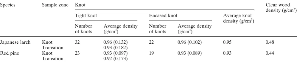
X-ray images for knot and transition zones were extracted from raw X-ray images of Japanese larch and red pine. Each density was obtained by converting each cell of the partial image for each zone. Table 2 shows the statistics of knot densities for two of the species tested. The densities of the knot and transition zones for two types of knots – tight knots and encased knots – were calculated using Beer’s Law. The X-ray image for the transition zone of the encased knot could not be extracted because the width of the transi-tion zone was too small. The average density was 0.95 g/cm3
for Japanese larch and 0.93 g/cm3
for red pine. Average
densities were approximately double the density of clear wood.12
A t-test was carried out to investigate the similarity of transition zone density to knot density. It was hypothesized that there is no difference between knot density (m1) and
transition zone density (m2): null hypothesis H0 : m1= m2
A two-tailed test with a signifi cance level of 0.10 was conducted. If a test statistic is larger than the P-value, H0 is
rejected. However, the two-tailed test showed that the densities of knot and transition zone were not different from each other in terms of a 10% signifi cance level (H0
accepted, Table 3). When the X-ray image was observed by the naked eye, the transition zone and knot were not identifi ed. This was considered to be caused by the similarity in density. Because the density of the transition zone is similar to knot density, the average density was used for the input variable of KDR calculation.
Verifi cation of KDR evaluation method
Comparison of KDRx and KDR1
To verify the proposed KDR method, KDRx and KDR1
were compared (Fig. 8). The KDRx predicted by the
pro-posed method commonly overestimated the KDR1. It was
speculated that the dense transition zone caused this over-estimation. The density of the transition zone is similar to the knot density (see Tables 2 and 3). This overestimation was prominent for low values of KDR1. A cell with a low
Fig. 7a, b. Relationship between
the density prediction by X-ray radiation and air-dry density.
a The 10-mm-thick specimens. b The 38-mm-thick specimens
Table 2. Knot density for two tree species
Species Sample zone Knot Clear wood
density (g/cm3)
Tight knot Encased knot Average knot density (g/cm3)
Number of knots
Average density (g/cm3)
Number of knots
Average density (g/cm3)
Japanese larch Knot 32 0.96 (0.132) 22 0.96 (0.102) 0.95 0.48 Transition 0.93 (0.182)
Red pine Knot 23 0.93 (0.097) 19 0.93 (0.089) 0.93 0.44 Transition 0.92 (0.173)
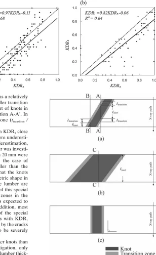
KDR1, for example, section B-B’ in Fig. 9a, has a relatively
large transition zone. Section B-B’ has a smaller transition zone than section A-A’; however, the amount of knots in section B-B’ is much smaller than that in section A-A’. In low KDR1 cells, the ratio of the transition zone (ttransition /
tknot, Fig. 9a) is relatively large.
In the case of Japanese larch, the cells with KDR1 close
to 1.0 were not overestimated; rather, they were underesti-mated (Fig. 8a). To fi nd the cause of this underestimation, the diameter of knots in appearance of lumber was investi-gated. The knots with diameters smaller than 20 mm were ignored in knot diameter measurement. In the case of Japanese larch, 99.4% of knots were smaller than the lumber thickness of 38 mm. This indicates that the knots with KDR1 close to 1.0 have a special geometric shape in
that the knot axis and the wide face of the lumber are almost at a right angle (Fig. 9c). In the case of this special knot geometry, the cells had no transition zones in the X-ray path; therefore, no overestimation was expected to occur in cells with KDR1 close to 1.0. In addition, most
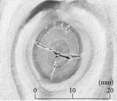
knots contained cracks (Fig. 10). Because of the special knot geometry found in the knots with cells with KDR1
close to 1.0, the reduction in X-ray attenuation by the cracks caused the cells with larger KDR1 values to be severely
underestimated.
In the case of red pine, however, it has larger knots than Japanese larch. In the knot diameter investigation, only 43.4% of red pine knots were smaller than the lumber thick-ness of 38 mm. Even though the knot axis and wide face were not at a right angle, a KDR1 value of 1.0 can exist
(section C-C’ in Fig. 9b). From these statistics of knot diam-eter, it can be inferred that the knots with larger KDR1
Fig. 9a–c. Cross-sectional views of different shapes of knots and the
Fig. 10. Example of knot containing cracks (Japanese larch)
values do not have a special geometry but have various geometries. Even though some cells may be underestimated due to cracks found in knots, no overall tendency for under-estimation was found (Fig. 8b).
Comparison of KDRx and KDR2
Because it was speculated that the transition zone would cause overestimation of KDR1, the KDRx value was
com-pared from the ratio of the knot and transition zone to the lumber thickness, KDR2. Figure 11 shows strong
relation-ships between KDRx and KDR2 for Japanese larch and red
pine, with R2
values of 0.87 and 0.83, respectively. The slope of the regression curve was close to 1.0 (dashed line). These results demonstrated that the proposed knot depth ratio prediction method is more suitable for evaluating KDR2
including the transition zone. Unfortunately, it cannot predict the ratio of knot in lumber thickness, and it involves transition zone as well as knot.
Even though redefi ning the KDR increases its accuracy, the misleading effect of cracks in knots, as in the Japanese larch specimens, still remains (Fig. 11a) and these errors are expected to occur in the analysis of other species containing small-diameter knots.
Prediction of ratio of knot area to cross-sectional area
Generally, it was assumed that knots reduce the effective cross-sectional area with regard to strength. Therefore, the relative ratio of knot was targeted for prediction. Because the KDR method gives the KDR values for knot zone including transition zone, the knot area ratio predicted by X-ray also contains the transition zone area.
The ratio of knot and transition zone area to the cross-sectional area was calculated from X-ray image analysis. The predicted area ratio (ARx) was compared with the real
area ratio (ARreal) defi ned as the ratio of knot and transition
zone area to the gross cross-sectional area.
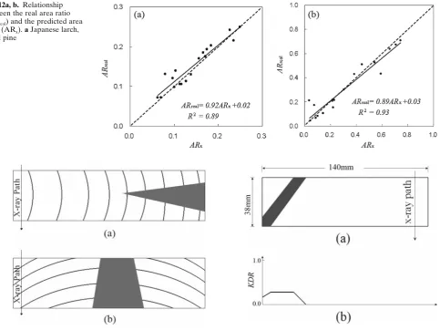
Figure 12 shows the relationship between the predicted area ratio and the actual area ratio, which is more successful than the KDR prediction. It was speculated that the annual rings cause the increase of coeffi cient of determinant. There are various geometries of annual rings due to the sawing method, including edge grain and fl at grain lumber (Fig. 13). If an X-rays pass through the tangential direction in edge grain lumber (Fig. 13a), the latewood and earlywood can be identifi ed in the X-ray image because latewood density is higher than that of earlywood. If latewood and knot exist together in the path of X-rays, the X-ray image analysis would overestimate the KDR value; conversely, earlywood causes it to be underestimated. Fortunately, late-wood and earlylate-wood coexist in a repeated fashion. If a cross section has cells that have been overestimated due to late-wood, it may also have the underestimated cells. It was considered that the extent of underestimation and overes-timation was nearly identical in a cross section. The effect of the repeated underestimations and overestimations caused by latewood and earlywood is thought to be mini-mized by their cancellation of each other.
Ultimately, it can be concluded that X-rays can be used to quantify knot area in a cross section, considering the R2
values of 0.89 for Japanese larch and 0.93 for red pine, even though the different density of latewood and earlywood affects the KDR calculation and reduces the accuracy. Because the KDRx value involves transition zone, the area
ratio predicted by X-ray image analysis also includes the transition zone area as well as knot area.
Fig. 11a, b. Relationship
between KDRx and KDR2,
which is the ratio of knot and transition zone to lumber thickness. a Japanese larch,
Even though this method cannot provide the exact location of knots in 38 mm of thickness (Fig. 14), the KDR method allows the evaluation of the knot area in a certain cross section and to identify the exact location of knot in a 140-mm width. In additional, this method requires only a single X-ray radiation. This differs from computed tomography, which uses a number of X-ray radiations.
In order to use the KDR evaluation method for grading or predicting strength, further studies on the relationship between strength and KDR are required, because the KDR values involve the transition zone as well as knots.
Conclusions
In this study, the knot depth ratio (KDR) evaluation method was proposed. This method was developed to quantify the geometric amount of knots in a cross section, using a single-pass X-ray radiation. To verify the proposed method, the KDR values for 38-mm-thick lumber were evaluated. After comparing the predicted KDR values with the real KDR values measured by observing the cross section, the conclusions are:
1. X-rays cannot distinguish between knot and transition zone because the density of the transition zone is similar to that of the knots.
2. The KDR method can quantify the ratio of knot involving transition zone to lumber thickness. The KDR values for Japanese larch and red pine specimens were predicted by the proposed method with R2
correlations of 0.87 and 0.83, respectively. However, underestimation of KDR caused by cracks in the knots still remains and further studies for various species with small-diameter knots are required.
3. In the KDR evaluation, the difference of density between latewood and earlywood in the same path of the X-rays causes estimation discrepancies. However, when the ratio of knot area to cross-sectional area was calculated using KDR information, the discrepancies were effec-tively canceled out because latewood and earlywood are repeated. Evaluation of the area ratio using KDR infor-mation increased the correlation between the predicted KDR and the real KDR with R2
values of 0.89 and 0.93 for Japanese larch and red pine, respectively.
Acknowledgments This study was carried out with the support of
Forest Science and Technology Projects (Project No. S120708L1001104) provided by the Korea Forest Service.
Fig. 13a, b. Geometry of the annual ring and the knot according to
sawing type. a Edge-grain lumber, b fl at-grain lumber
Fig. 14a, b. Geometric meaning of the knot depth ratio evaluation
References
1. Riberholt H, Madsen PH (1979) Strength of timber structures, measured variation of the cross sectional strength of structural lumber. Report R 114, Structural Research Laboratory, Technical University of Denmark
2. Schniewind AP, Lyon DE (1971) Tensile strength of redwood dimension lumber II. Prediction of strength values. Forest Prod J 21:45–55
3. Johansson CJ, Brundin J, Gruber R (1992) Stress grading of Swedish and German timber. A comparison of machine stress grading and three visual grading systems. Swedish National Testing and Research Institute, SP Report 1998:38
4. Machado JS, Sardinha RA, Crus HP (2007) Feasibility of auto-matic detection of knots in maritime pine timber by acousto-ultra-sonic scanning. Wood Sci Technol 38:277–284
5. Baradit E, Aedo R, Correa J (2006) Knots detection in wood using microwaves. Wood Sci Technol 40:118–123
6. Gerhards CC (1982) Effect of knots on stress waves in lumber. Research Paper FPL-RP-384. USDA Forest Products Laboratory, Madison, WI, USA
7. Hu C, Tanaka C, Ohtani T (2004) Location and identifying sound knots and dead knots on sugi by the rule-based color vision system. J Wood Sci 50:115–122
8. Lam F, Barrett D, Nakajima S (2005) Infl uence of knot area ratio on the bending strength of Canadian Douglas fi r timber used in Japanese post and beam housing. J Wood Sci 51:18–25
9. Madsen B (1992) Structural behaviour of timber. Timber Engi-neering, pp 52–79
10. Institute of Isotopes of the Hungarian Academy of Sciences (1986) Industrial application of radioisotopes. Elsevier, Amsterdam, pp 232–239
11. Kim KM, Lee SJ, Lee JJ (2006) Development of portable X-ray CT system I – evaluation of wood density using X-ray radiography. J Korean Wood Sci Technol 34:15–22
12. Sahlberg U (1995) Infl uence of knot fi bers on TMP properties. TAPPI J 78:162–168
13. Oh JK, Kim KM, Shim K, Park JH, Kim WS, Yeo H, Lee JJ (2007) Prediction of bending performance for Japanese larch lumber: X-ray scanning. Proceedings of the Korean Society of Wood Science and Technology Annual Meeting, Yeosu, pp 71–72
14. Kim KM, Lee SJ, Lee JJ (2006) Development of portable X-ray CT system II – CT image reconstruction of wood using density distribution. J Korean Wood Sci Technol 34:23–31
15. Lee SJ, Kim KM, Lee JJ (2006) Application of the X-ray CT tech-nique for NDE of wood in fi eld. Key Eng Mater 321–323:1 172–1176
16. Rojas G, Condal A, Beauregard R, Verret D, Hernandex RE (2006) Identifi cation of internal defect of sugar maple logs from CT images using supervised classifi cation methods. Holz Roh Werkst 64:295–303
17. Korean Standards Association (2002) Softwood structural lumber, KS F 2162