A new evaluation function for face image enhancement in unconstrained environments using metaheuristic algorithms

(1)

R E S E A R C H

Open Access

A new evaluation function for face image

enhancement in unconstrained

environments using metaheuristic

algorithms

Muhtahir Oloyede

*

, Gerhard Hancke, Hermanus Myburgh and Adeiza Onumanyi

Abstract

Image enhancement is an integral component of face recognition systems and other image processing tasks such as in medical and satellite imaging. Among a number of existing image enhancement methods, metaheuristic-based approaches have gained popularity owing to their highly effective performance rates. However, the need for improved evaluation functions is a major research concern in the study of metaheuristic-based image enhancement methods. Thus, in this paper, we present a new evaluation function for improving the performance of metaheuristic-based image enhancement methods. Essentially, we applied our new evaluation function in conjunction with metaheuristic-based optimization algorithms in order to select automatically the best enhanced face image based on a linear combination of different key quantitative measures. Furthermore, different from other existing evaluation functions, our evaluation function is finitely bounded to determine easily whether an image is either too dark or too bright. This makes it better suited to find optimal solutions (best enhanced images) during the search process. Our method was compared with existing metaheuristic-based methods and other state-of-the-art image enhancement techniques. Based on the qualitative and quantitative measures obtained, our approach is shown to enhance facial images in unconstrained environments significantly.

Keywords:Pre-processing, Image enhancement, Metaheuristic algorithm, Unconstrained environments

1 Introduction

Pre-processing in face recognition systems involves enhancing an input face image in order to improve its quality by making more facial features in the image visible. Pre-processing enhances the performance of face recogni-tion techniques [1, 2]. Further, the pre-processing stage amends distorted images and acquires regions of interest in an image for onward feature extraction. One important pre-processing task is image enhancement, which is essen-tial to improve the performance of face recognition systems. However, most face recognition systems do not often incorporate face image enhancers in their designs, and whenever they do incorporate them, these are often less effective methods prior to the recognition process [3,

4].There are many image enhancement methods used in

face recognition systems today. These methods have their pros and cons. Some recent methods transform an input image in order to achieve a more detailed or less noisy output image [5,6]. In this regard, an image enhancement technique (IET) is considered effective if it is self-adaptive, i.e., if it adjusts its parameters to improve its performance automatically over different images. An IET must enhance an input image without introducing overstretching, excessive brightness, or loss of important features [7]. They should be simple with low computational complexity [8,9]. These qualities are desired in a typical IET.

However, in face recognition systems, the quality of face images in unconstrained environments may be notably degraded for many reasons such as lighting conditions, i.e., in dark or too bright environments. Also, various facial expressions, change of pose, occluded faces, and other fa-cial conditions may change the appearance of face images by hiding important features in the face [10]. Some IETs * Correspondence:[email protected]

Department of Electrical Electronic and Computer Engineering, University of Pretoria, Pretoria, SA 0002, South Africa

(2)

have been developed for various image-processing tasks; however, researchers have done minimal work concerning the development of IETs for face recognition in uncon-strained environments. Further, most IETs often produce less enhanced outputs or unnatural effects and over enhancement in some cases that negatively affect the performance of face recognition systems. For these reasons, experts need to develop better IETs to improve further the performance of face recognition systems.

In terms of existing IETs, the histogram equalization (HE) method is a popular and simple approach for image enhancement [11, 12]. It works by adjusting the image’s contrast either by increasing or decreasing the global con-trast of the image, especially when the image is character-ized by close contrast values [13]. It operates by spreading the intensities of image pixels based on the information from the entire image. This results in conditions where low occurring intensities are transformed and fused with neigh-boring high occurring intensities, thus leading to over en-hancement [14]. Further, mean shift issues may arise in such a situation, which maintains the image’s brightness and limits the performance of HE. The bi-histogram equalization (BHE) method was developed to address this problem [15], and it displayed better performance while maintaining the quality of the original image. However, the BHE is limited when the image pixel distribution is not symmetrical. Other methods such as the gamma correction and logarithm transformations have been used with lower computational complexities. However, they cannot manage complex illumination differences. Furthermore, other ex-tensions of HE have been proposed such as the block-based histogram equalization, oriented local histogram equali zation, and adaptive histogram equalization (AHE) methods. Nevertheless, these methods typically underper-form in face recognition tasks, particularly in complex illu-mination conditions. This poor performance occurs because these methods rescind the entire distribution, which may contain important image characteristics [10].

Singh and Kapoor [16] presented an exposure-based sub-image histogram equalization method for contrast enhancement in low exposure grayscale images. Their method obtains thresholds, which are computed in order to split the original image into sub-images of various inten-sity levels. To control the enhancement rate, the histogram is clipped utilizing a threshold value as an average number of gray-level occurrences. Their method performed better than other conventional histogram equalization approaches. However, their approach does not adjust the level of enhancement, thereby resulting in darker or brighter en-hanced images. Zhuang and Guan [17] used the mean and variance-based sub-image histogram equalization method to increase the contrast of the input image with brightness while retaining important features. However, because some IETs produce over-enhanced images and artifacts, Hussain

et al. [8] proposed a dark image enhancement approach where local transformation of the image pixels is consid-ered. The experiments in [8] showed that their method im-proved satisfactorily the quality of images. However, artifacts were present in the images. Reddy et al. [12] pre-sented the dynamic clipped histogram equalization for en-hancing low contrast images. Their approach selects a clipped level at the occupied bins and conducts histogram equalization on the clipped histogram to produce the out-put image. Reddy’s method uses three variants of the occu-pied bin space to enhance the low-contrasted dark, bright, and gray images. Shi et al [2] presented a dual channel prior-based method for nighttime low illumination image enhancement using a single image that is based on two existing image priors i.e., bright and dark priors. They used the bright channel prior to obtain the initial transmission estimate and used the dark prior as a complementary channel to adjust any wrong transmission estimate produced by the bright channel prior.

Linear contrast stretching (LCS) is an IET that uses lin-ear transformation to increase the dynamic range of gray levels present in an original image [18]. LCS improves the contrast grade of an image; however, the LCS’s threshold value must be manually configured. If a wrong threshold value is used, the quality of the enhanced image will be low. Since no universal standard exists for image quality assessment, it becomes difficult to improve on an image by simply stretching its histogram or utilizing simple gray-level transformations [19,20].

Thus, to solve these general issues, particularly when computers need to decide autonomously how good an enhanced image is, researchers have recently proposed methods based on evolutionary computation and meta-heuristic optimization algorithms [21]. Metaheuristic algo-rithms are generally used to finding solutions involving non-linear optimization tasks. Munteanu and Rosa [5] pio-neered the application of metaheuristic algorithms for image enhancement. They used an evaluation function (EF) to select automatically the most appropriate enhanced image without requiring human intervention. Thus, they proposed a novel EF and an evolutionary algorithm to globally search for the best enhanced image from among a solution space of candidate-enhanced images.

(3)

using an incomplete beta function as the transformation function. Three factors, namely the entropy value, thresh-old, and the probability density of the image, were used in [13] to measure the quality of the enhanced image. They evaluated and compared their approach to other IETs and showed improved performances. However, their model does not select always the most enhanced image, which necessitates the need for better methods.

Following in this paper, we present a metaheuristic-based IET for enhancing face images in an automatic and more effective manner than previous approaches. The primary contributions of our research are as follows:

1. We present a new EF as a component within the IET for face images.

2. We present a defined scaling mechanism for the EF in order to ensure that extreme values of an enhanced image depict either completely dark or completely white images.

3. Our proposed IET exhibits stability in selecting the most enhanced image based on both qualitative and quantitative measures.

4. Extensive quantitative and qualitative experiments were carried out to compare different existing standard EFs.

5. A comprehensive evaluation of the different standard metaheuristic-based algorithms was carried out.

The remainder of the paper is organized as follows: Section 2 discusses the proposed IET, where the related functions used are highlighted. Section 3 describes the data samples and the performance evaluation used. Section 4 discusses the experiments and simulation re-sults compared with various state-of-the-art algorithms. Section 5 concludes the research work giving highlights of the merits of our proposed algorithm and scope for future research work.

2 Proposed method

2.1 Image enhancement technique

An IET uses an effective transformation function to effi-ciently map the intensity values of an original input image in order to produce an enhanced output image [23]. In metaheuristic-based methods, this process requires that an EF selects automatically the optimal enhancement parame-ters of a transformation function in order to appropriately enhance an image [24]. This section describes the trans-formation function used in our research, our proposed EF, and the metaheuristic algorithm that we considered.

2.2 Transformation function

Generally, the process of enhancing images in the spatial domain requires the use of a transformation function,

which assigns new intensity values to each image pixel of the original image in order to produce an enhanced image. Local enhancement approaches apply transform-ation functions based on the gray-level distribution in the neighborhood of every pixel in a given input image. In our research, we used the transformation function proposed by Munteanu and Rosa in [5]. Munteanu’s ap-proach applies a transformation function,T, to each pixel at a location (i, j) using the gray-level intensity of the pixel within the input image, f(i, j), and converts these intensities to another value,g(i, j), i.e., the gray-level in-tensity of the output image. The horizontal and vertical size of the image is denoted as Hsize and Vsize, respect-ively. Hence,Tis defined according to [5] as:

g ið Þ ¼;j T f ið ð Þ;jÞ ¼k M

σð Þ þi;j b

½f ið Þ;j−cm ið Þ;j þm ið Þ;ja

ð1Þ

wherem(i,j) andσ(i,j) represent the mean and standard deviation of the gray scale image obtained for the pixels in the neighborhood centered at (i,j). The global mean,

M, of the original image is computed as M¼PHsize−1 i¼0

PVsize−1

j¼0 fði;jÞ. The parameters a, b, c, and k in Eq. (1) have the following effects: Parameter a introduces a brightening bias in the output image based on the last termm(i,j) in Eq. (1). It enables further control over the amount of smoothening effect required in the output image. Parameter b ensures that a zero-standard devi-ation value in the local neighborhood pixels does not have a huge whitening effect on the final output image. Thus, by its introduction, the denominator component in Eq. (1) typically remains nonzero. Parameter callows only a fraction of the mean,m(i,j), to be subtracted from the original pixels of the input image. The parameter c controls the degree of darkening introduced in the out-put image. Parameterkis introduced to create a fair

bal-ance between pixels existing in the mid-range

boundaries of the gray scale. Essentially, these pixels are prevented from being either too dark or too white dur-ing the enhancement process. The followdur-ing parameter values were noted to be highly effective based on an ex-tensive empirical parameter-tuning exercise conducted in our work: 2≤a≤2.5, 0.3≤b≤0.5; 0≤c≤3, and 3≤

k≤4. These values formed the limits of the constraints used in the optimization process of our method.

2.3 Evaluation function

(4)

describe as follows: Firstly, we began by identifying par-ticular key metrics in the literature that suitably describe how well an image is enhanced or not. We considered as many metrics as possible, which differentiates our model from existing models in the literature. Secondly, we introduced the concept of normalizing the metrics in our model in order to provide a bound for our method. This innovation made it possible to define a linear func-tion that differs from existing funcfunc-tions in the literature. Interestingly, by this innovation, our method defines specific boundaries for images in very black and very white regions. These clear boundaries further enable an optimization algorithm to find better solutions in a well-defined range. Thirdly, we investigated three differ-ent optimization methods in order to use the best method, which led to the choice of the cuckoo search optimization algorithm. We present evidence of its per-formance in Section4.

Thus, in developing our EF, and similar to [25], we quan-tified the following qualities of a well-enhanced image as follows: A well enhanced image should have a higher num-ber of edge pixels than the original image. Furthermore, an enhanced image is expected to have a higher measure of in-formation than the original image. This measure of infor-mation can be quantified using an entropic metric such as the histogram of the image. This approach is similar to the information measure used in the histogram equalization technique. Similarly, more pixels belonging to the foground objects in an enhanced image should be better re-vealed than in the original image. An enhanced image should contain less alien artifacts than the original image. Based on the above qualities of an enhanced image, we propose a new EF that comprises of different performance metrics. These metrics, which are used to measure the qualities mentioned above, include the number of edge pixels, number of foreground pixels, entropic measure, and the peak signal-to-noise ratio (PSNR).

We describe the process of our EF as follows: First, the number of edge pixels,Ng, in the enhanced image is com-puted. To achieve this, a Sobel threshold,Tf, is automatically computed from the original image, f(i,j), using the Sobel edge detector. This threshold,Tf, is then used in the Sobel edge detector to obtain the edge intensities, Eg(i,j), of the enhanced image. In addition to being invariant,Tfwas con-sidered in our EF for computingEg(i,j) in order to ensure a fair comparison between the original image and the different instances of the enhanced image. Thus, the number of edge pixels,Ng, in the enhanced image is obtained as:

Ng¼

XH

i¼1

XV

j¼1

Egð Þi;j ð2Þ

Secondly, the number of pixels, ϕg, belonging to the foreground objects ing(i,j) is computed. To achieve this,

the variance ϑg(i,j), of g(i,j), and the variance ϑf(i,j), of

f(i,j), are computed within a neighborhood (window)

having n×n pixels. A threshold value, ηf, is automatic-ally computed for ϑf(i,j) using Otsu’s threshold algo-rithm. A representation, Dg(i,j), revealing pixels belonging to the foreground objects in the enhanced image is obtained as:

Dgð Þ ¼i;j

1 ifϑgð Þi;j ≥ηf 0 if otherwise 8

<

: fori¼1;2;…;H;j¼1;2;…;V: ð3Þ

Thus,ϕg, is obtained as

ϕg ¼

XH

i¼1

XV

j¼1

Dgð Þi;j ð4Þ

Thirdly, an entropic measure,βg, of g(i,j) is computed as

βg¼

−X

m

ΩmlogðΩmÞ forΩm≠0

0 forΩm≠0

8 < :

ð5Þ

whereΩmis the frequency of pixels having gray levels in

the histogram bin,m= 1,…, 256. The PSNR,ρg, ofg(i,j)

is obtained as

ρg ¼10 log10

L−1 ð Þ2

MSE

" #

ð6Þ

where L is the maximum pixel intensity value in g(i,j) and MSE is given as

MSE¼ 1

HV XH

i¼1

XV

j¼1

f ið Þ;j−gði;jÞ

j j2 _ð₇_Þ

Based on the parameters computed in Eqs. (2)–(7), a new EF,Ε, is proposed as

Ε¼1−exp − ρg 100

þN_Hgþ_Vϕgþβg

8 ð8Þ

(5)

2.4 Metaheuristic algorithm

Metaheuristic optimization algorithms generally find so-lutions for highly non-linear optimization tasks [26]. They follow an iterative process that directs a subordin-ate heuristic by automatically fusing various ideas to ex-plore a solution search space. Learning strategies are utilized to arrange information in order to find efficient optimal solutions. There are different types of metaheur-istic algorithms known to be effective, such as the par-ticle swarm optimization (PSO), genetic algorithm (GA), and the cuckoo search optimization (CSO) algorithms. In our research work, the CSO was used following an extensive comparison of the different metaheuristic algo-rithms as presented in the result section (see Section

4.2). The CSO algorithm was developed in [27], and it is among the most recent metaheuristic algorithms used for global optimization, with a look-alike process of the brood parasitic behavior of certain cuckoo species. The CSO was considered for its simplicity, fast convergence, and for its useful capability proven over series of experi-ments carried out in [28]. These attributes are essential requirements, which we considered worthwhile in order to enhance the contrast of images. The CSO algorithm based on Levy flight was applied in our work for search-ing new solutions based on the model given as:

aiðcþ1Þ¼aið Þc þαLevyð Þλ ð9Þ

whereai(c+ 1)depicts the latest solutions for a cuckoo,i,

using flight function, with λ representing the Levy walk parameter, α represents the step size associated to the scale of the problem of interest, and ⊗ product repre-sents entry wise multiplication. The Levy flight produces a random walk while the arbitrary step length is derived from a Levy distribution as Levy ∼u=t−λ, (1 <λ≤3). Generally, the process of the CSO is described as fol-lows: every egg present in a nest denotes a solution and a cuckoo egg depicts a new solution. The purpose is to utilize the latest and supposedly better solutions, i.e., cuckoo to swap the less efficient solutions in the nests [27]. The adoption of the CSO in our work considers the situation for just an egg, as we are interested in only one solution. Table 1 describes the algorithmic process in the CSO. In the next section, we describe the entire flow process involved in our proposed image enhance-ment method based on an integration of the transform-ation function, our proposed EF, and the CSO algorithm.

2.5 Summary of the proposed image enhancement algorithm

In this section, we provide a summary of our proposed image enhancement method as stipulated in Table 1. Typically, the inputs to our method are the original image to be enhanced and the range of values describing

the lower and upper constraints of each parameter. The process converts the original image to its corresponding gray scale image. This gray scale image is passed to the CSO algorithm where the entire optimization process selects the best enhanced image. Essentially, we describe the process involved in a single iteration of the CSO al-gorithm. However, the iteration typically continues until a stopping criterion is met or there is no further change in the fitness value.

Firstly, the original gray scale image is subjected to the transformation function in Eq. (1) to obtain a supposed enhanced image. The transformation function is applied based on a set of initial parameter values selected by the CSO algorithm in a random manner. These parameter values are used in the transformation function in order to obtain a supposed enhanced image. This enhanced image is then passed to the EF were a specific value is computed for the enhanced image as described in

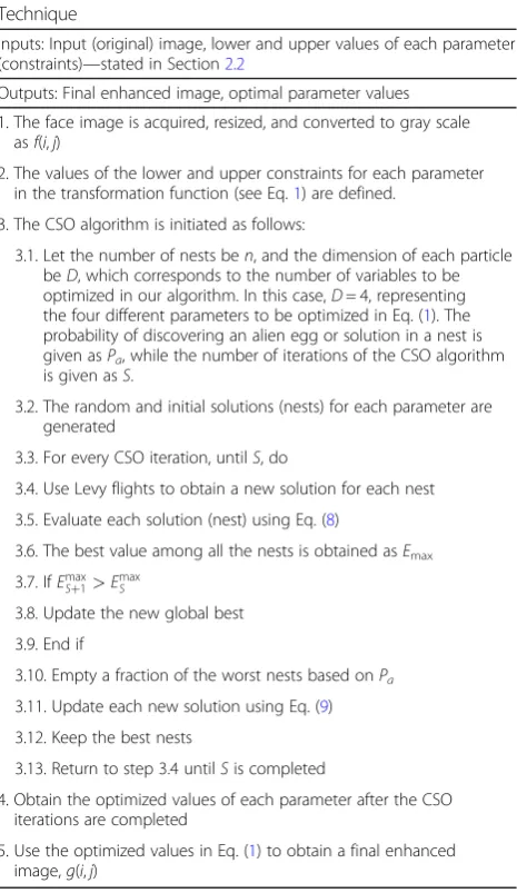
Table 1Steps involved in the Proposed Face Image Enhancement

Technique

Inputs: Input (original) image, lower and upper values of each parameter (constraints)—stated in Section2.2

Outputs: Final enhanced image, optimal parameter values

1. The face image is acquired, resized, and converted to gray scale asf(i,j)

2. The values of the lower and upper constraints for each parameter in the transformation function (see Eq.1) are defined.

3. The CSO algorithm is initiated as follows:

3.1. Let the number of nests ben, and the dimension of each particle beD, which corresponds to the number of variables to be optimized in our algorithm. In this case,D= 4, representing the four different parameters to be optimized in Eq. (1). The probability of discovering an alien egg or solution in a nest is given asPa, while the number of iterations of the CSO algorithm

is given asS.

3.2. The random and initial solutions (nests) for each parameter are generated

3.3. For every CSO iteration, untilS, do

3.4. Use Levy flights to obtain a new solution for each nest

3.5. Evaluate each solution (nest) using Eq. (8)

3.6. The best value among all the nests is obtained asΕmax

3.7. IfΕmax

Sþ1>ΕmaxS

3.8. Update the new global best

3.9. End if

3.10. Empty a fraction of the worst nests based onPa

3.11. Update each new solution using Eq. (9)

3.12. Keep the best nests

3.13. Return to step 3.4 untilSis completed

4. Obtain the optimized values of each parameter after the CSO iterations are completed

(6)

Section 2.3. This EF value is one of several possible values computed for different enhanced images belong-ing to a population of possible enhanced images. Thus, each enhanced image in the population is subjected to the transformation function using different sets of par-ameter values and then passed to the EF to obtain a fit-ness value. The best (or largest) EF value from among a population of different enhanced images is selected per generation (or iteration). The iteration proceeds until no better value is obtained. Thus, the enhanced image that produces the highest EF value after several number of it-erations (or generation) is outputted as the best en-hanced image.

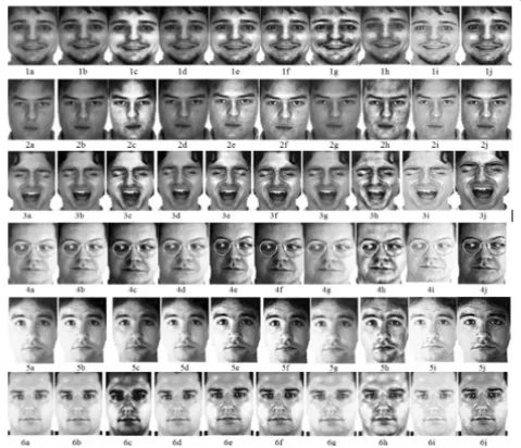
3 Performance evaluation and data samples used In our work, we enhanced face images in unconstrained environments. Thus, we used face images obtained from three different standard benchmark face datasets, i.e., the AR face database [29], Yale face dataset (YF), and the Olivetti research laboratory face dataset (ORL). Face images affected by different lighting conditions, different facial expressions, and different pose variations were se-lected from each face database. The lighting conditions

used were from the right, left, and both sides. Further, for the different facial expressions, face images with smile, anger, and scream were selected.

We describe the protocol used to select the represen-tative images considered in the evaluation of our method and other state-of-the art approaches as follows: Essen-tially, six different images were selected based on our protocol. Firstly, since our research focused on facial im-ages and their constraints, we used six different types of representative facial conditions in unconstrained envi-ronments, namely smile, anger, scream, right light illu-mination, left light illumination, and both side illumination. Secondly, we categorized all images in each dataset into these six different facial conditions. Thirdly, one representative image from each category was ran-domly selected, thus accounting for the six different images presented in Section4per dataset.

The effectiveness of an IET can be measured qualita-tively by visualizing the enhanced output image. How-ever, it is also required to describe quantitatively the degree of enhancement of an image. We describe the following metrics used to assess quantitatively the meas-ure of enhancement of an image. The metrics considered are number of edges, number of pixels in the fore-ground, entropic measure, PSNR, and absolute mean brightness error (AMBE), which are defined in the fol-lowing sub-sections.

3.1 Number of edges

The number of edges produced by an IET must provide a more substantial number of edges on the enhanced image as compared to the original input image. A higher number of edges on the enhanced image are desired as compared to the input image. The number of edges Ng can be obtained as stated in Eq. (2).

3.2 Number of pixels in the foreground

An effective IET must be able to reveal more pixels that belong to the foreground object in the enhanced image

Fig. 1Choice of CSO parameter

a

b

c

(7)

as compared to the original image. Hence, a higher value of the number of pixels in the foreground is desired to quantify the effectiveness of an IET. The number of pixels in the foreground ϕgcan be obtained as stated in Eq. (4).

3.3 Entropic measure

An entropic measure is regarded as the process of quan-tifying the details of information in the image. The larger the entropic measure value, the more detailed an en-hanced image will be. Also, the entropic value of an image is independent of a different image because com-parison is done on the same image before and after the processing [30]. The entropic measure of the enhanced imageβgcan be obtained as stated in Eq. (5).

3.4 PSNR

An IET must not only have the ability to improve the images but also control the level at which artifacts is introduced into the enhanced image, i.e., the level of noise should not be increased during the enhance-ment process. The PSNR ρg is used to evaluate the increase in quality between the original and the en-hanced image [31]. The PSNR value can be obtained as stated in Eq. (6).

3.5 AMBE

The AMBE, ξ, is generally used to measure the rate at which the mean brightness is preserved, which can be represented mathematically as in Eq. (10). It shows the change in mean brightness value between the original and the enhanced image. Furthermore, the mean bright-ness of the original and enhanced image can be calcu-lated as shown in Eqs. (11) and (12), respectively. Thus, a lower AMBE value is desired, while a zero AMBE value is considered the ideal result.

ξ¼jδðf ið Þ;jÞ−δðg ið Þ;jÞ j; ð10Þ

δðf ið Þ;j Þ ¼_HV1 X i

X

j

δðf ið Þ;jÞ; ð11Þ

δðg ið Þ;jÞ ¼_HV1 X i

X

j

δðg ið Þ;j Þ ð12Þ

where δ(f(i,j)) depicts the mean brightness of the ori-ginal image andδ(g(i,j)) represents the mean brightness of the enhanced image.

4 Simulation results and discussion

In this section, we discuss the effects of various experi-ments carried out in our research work. Firstly, an ex-periment to determine the choice of appropriate CSO parameters was conducted. Then, simulations using dif-ferent metaheuristic algorithms were conducted to as-sess the respective performances of each algorithm based on the fitness value and time of convergence. Fur-thermore, we carried out experiments to compare our function with other EFs using the CSO algorithm in order to verify the effectiveness of our proposed EF. Finally, to confirm the efficacy of our image enhance-ment method, quantitative and qualitative comparisons were conducted based on standard performance metrics across different standard benchmark datasets.

Table 2Comparison of the different metaheuristic algorithm

with our proposed EF based on all the performance evaluation metrics

d

Fig. 7Qualitative comparison of the different evaluation function with the CSO algorithm on Image 2.aOriginal.bMunteanu + CSO.cYe + CSO.

(9)

4.1 Choice of CSO parameter

To effectively select appropriate values of the parameter, Pa, for the CSO algorithm, an experiment with different values ranging between Pa = 0.1 to 1.0 was conducted. Results were plotted based on the number of iterations and the fitness value. It is seen in Fig.1 below that Pa = 0.2 converged the earliest. Hence, in our research, we selected Pa = 0.2.

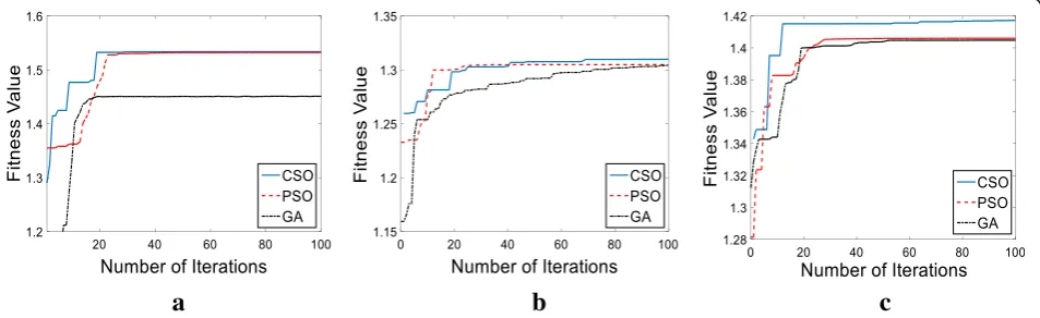
4.2 Evaluation of different metaheuristic algorithms

To confirm the selection of the metaheuristic algorithm used in our research, an evaluation of different meta-heuristic algorithms was carried out. The algorithms considered include the CSO, PSO, and genetic algorithm (GA) methods. The number of iterations for each meta-heuristic algorithm was set at 100, which we plotted against the fitness value for each metaheuristic algo-rithm. In order to avoid bias, we selected three different images from the AR dataset and evaluated the perform-ance of the different algorithms as shown in Fig.2.

In Fig.2, it is seen that across the different images la-beled (a), (b), and (c), the CSO algorithm outperformed other metaheuristic algorithms. For image 1, the fitness function value obtained by the CSO is 1.534; followed closely by the PSO at a fitness value of 1.532, and lastly the GA with a fitness value of 1.4509. For image 2, the fitness function of the CSO reached a value of 1.31, which is followed by the PSO value of 1.304 and GA ob-tained a value of 1.302. Similarly, evaluating the different

algorithms on image 3, the CSO algorithm achieved the highest fitness function value of 1.417, while being followed by the PSO algorithm with a fitness function value of 1.406, and lastly the GA with a fitness function value of 1.404. The convergence analysis of the different algorithms was also observed with the CSO algorithm converging the earliest across all images at the 20th, 63rd, and 95th iteration for images 1–3, respectively. Furthermore, as shown in Table 2, we compared the different metaheuristic algorithms based on our pro-posed EF using all the performance evaluation metrics such as the number of pixels in the foreground, num-ber of edges, PSNR, entropic measure, AMBE, and fitness value.

The various performance evaluation metrics are de-fined in Section 3. From Table2, the CSO algorithm in conjunction with our EF provided exciting and useful re-sults reported as follows for image 1; the number of pixels in the foreground value of 6026 was attained for the CSO outperforming PSO and GA with values of 4267 and 5806, respectively. Similarly, in image 3, the highest number of pixels in the foreground value of 4567 was attained using the CSO with our proposed al-gorithm, outperforming the values of 4318 and 4291 generated by PSO and GA, respectively. Furthermore, the values generated for the number of edges on the dif-ferent images by the CSO algorithm with the proposed EF outperformed all other techniques. This implies that the CSO algorithm with the proposed EF is able to

a

b

c

d

Fig. 8Qualitative comparison of the different evaluation function with the CSO algorithm on Image 3.aOriginal.bMunteanu + CSO.cYe +

CSO.dProposed + CSO

Table 3Quantitative comparison for different EFs

Metrics Munteanu + CSO (M_CSO) Ye + CSO Proposed + CSO

Im1 Im2 Im3 Im1 Im2 Im3 Im1 Im2 Im3

ϕg 1867 1082 2301 762 927 1935 2104 1116 4827

Ng 537 361 630 1314 1673 1719 2306 2057 3368

ρg 14.9 13.3 17.0 17.7 15.7 17.8 14.5 13.8 12.9

βg 7.8 7.7 7.7 7.8 7.6 7.8 7.8 7.7 7.8

ξ 0.1 0.1 0.0 0.0 0.0 0.0 0.0 0.1 0.0

(10)

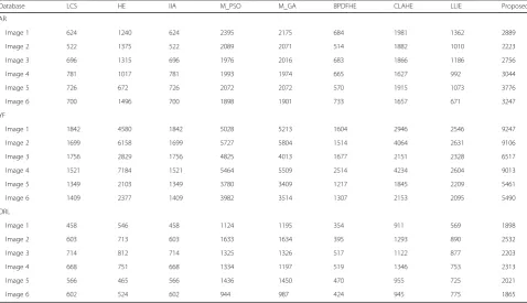
Table 4Number of pixels in the foreground value comparison between results obtained using different enhancement methods on standard benchmark face datasets

Database LCS HE IIA M_PSO M_GA BPDFHE CLAHE LLIE Proposed

AR

Image 1 451 1006 451 2565 2249 391 1560 977 3294

Image 2 399 1220 399 2407 2388 334 1248 655 2565

Image 3 937 2174 937 3582 3669 891 2660 1734 5424

Image 4 989 1572 989 3491 3475 740 2283 895 5956

Image 5 636 677 636 2902 2912 462 2134 961 6865

Image 6 383 887 383 2317 2324 190 651 371 3947

YF

Image 1 1308 9563 1308 5693 5955 950 1249 1439 13,117

Image 2 1515 13,388 1515 8914 9129 1359 1966 1175 17,694

Image 3 2285 6298 2285 8547 7003 2098 2010 3006 12,425

Image 4 1589 14,331 1589 7806 8105 1347 2004 1034 18,071

Image 5 1712 4731 1712 5936 5324 1508 1356 834 9751

Image 6 1887 5555 1887 6824 6080 1686 1515 1004 10,483

ORL

Image 1 482 489 482 1795 1909 333 1066 623 3873

Image 2 1938 2191 1938 5277 5279 1318 4209 2873 7618

Image 3 1784 2167 1784 3926 3928 1246 3218 2385 6499

Image 4 1438 1556 1438 3324 2877 1014 2658 1552 6248

Image 5 1330 1016 1330 4312 4353 1025 2513 1958 5946

Image 6 915 738 915 1792 1912 559 1240 1152 4705

Table 5Number of edge value comparison between results obtained using different enhancement methods on standard

benchmark face datasets

Database LCS HE IIA M_PSO M_GA BPDFHE CLAHE LLIE Proposed

AR

Image 1 624 1240 624 2395 2175 684 1981 1362 2889

Image 2 522 1375 522 2089 2071 514 1882 1010 2223

Image 3 696 1315 696 1976 2016 683 1866 1186 2756

Image 4 781 1017 781 1993 1974 665 1627 992 3044

Image 5 726 672 726 2072 2072 570 1915 1073 3776

Image 6 700 1496 700 1898 1901 733 1657 671 3247

YF

Image 1 1842 4580 1842 5028 5213 1604 2946 2546 9247

Image 2 1699 6158 1699 5727 5804 1514 4064 2631 9106

Image 3 1756 2829 1756 4825 4013 1677 2151 2328 6517

Image 4 1521 7184 1521 5464 5509 2514 4234 2604 9013

Image 5 1349 2103 1349 3780 3409 1217 1845 2209 5461

Image 6 1409 2377 1409 3982 3514 1307 2153 2095 5490

ORL

Image 1 458 546 458 1124 1195 354 911 569 1898

Image 2 603 713 603 1633 1634 395 1293 890 2532

Image 3 714 812 714 1325 1326 517 1122 877 2203

Image 4 668 751 668 1334 1197 519 1346 753 2313

Image 5 566 465 566 1436 1450 470 955 725 2021

(11)

Table 6Peak signal-to-noise ratio value comparison between results obtained using different enhancement methods on three different standard benchmark face datasets

Database LCS HE IIA M_PSO M_GA BPDFHE CLAHE LLIE Prop

AR

Image 1 23.135 17.921 23.135 14.430 15.239 27.1569 17.021 13.99 13.259

Image 2 21.184 15.375 21.848 12.396 12.392 34.8048 16.348 14.281 12.6282

Image 3 25.490 19.090 25.490 15.746 15.318 32.3678 18.724 13.833 12.437

Image 4 24.003 14.126 24.003 12.846 12.428 40.5588 16.8669 17.726 8.8844

Image 5 24.360 15.6500 24.360 14.5273 14.4144 40.5269 17.5406 17.654 9.147

Image 6 24.2599 9.8793 24.259 14.1864 14.17 29.9462 17.1313 21.347 8.244

YF

Image 1 27.071 12.472 27.071 14.101 13.269 34.115 23.451 26.014 8.069

Image 2 36.541 12.581 36.541 13.711 13.757 35.481 20.531 15.104 8.197

Image 3 37.271 17.085 37.271 13.207 6.607 37.806 21.755 23.831 9.759

Image 4 42.581 13.731 42.581 14.659 14.048 25.339 19.812 14.259 8.837

Image 5 39.031 18.110 39.030 2.2967 3.328 32.593 20.954 14.969 9.499

Image 6 35.343 16.072 35.343 13.392 5.065 37.973 21.706 17.007 9.027

ORL

Image 1 25.323 20.849 25.323 17.551 16.441 31.981 18.153 16.097 11.635

Image 2 26.787 22.484 26.787 14.861 14.831 41.335 16.407 14.606 10.258

Image 3 25.591 22.103 25.591 16.318 16.212 37.621 17.695 18.665 10.188

Image 4 23.788 19.598 23.788 15.441 16.947 33.865 17.825 18.590 10.523

Image 5 25.624 28.241 25.624 15.371 15.381 36.755 17.314 16.071 12.158

Image 6 22.703 21.727 22.703 18.523 18.139 32.633 17.743 15.356 11.829

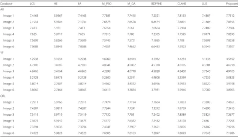
Table 7Entropic measure value comparison between results obtained using different enhancement methods on standard

benchmark face datasets

Database LCS HE IIA M_PSO M_GA BDPFHE CLAHE LLIE Proposed

AR

Image 1 7.4463 5.9567 7.4463 7.7381 7.7415 7.2321 7.8153 7.4387 7.7312

Image 2 7.1931 5.9504 7.1931 7.6573 7.6578 6.8574 7.6891 7.1804 7.8393

Image 3 7.413 5.931 7.413 7.6654 7.661 7.0664 7.7904 7.2489 7.7804

Image 4 7.635 5.9717 7.635 7.7815 7.786 7.2305 7.7595 7.0171 7.8593

Image 5 7.5609 5.8266 7.5609 7.5745 7.5721 7.1865 7.708 7.0508 7.8258

Image 6 7.0688 5.8843 7.0688 7.4651 7.4632 6.6483 7.5923 6.3949 7.3507

YF

Image 1 4.2938 3.1034 4.2938 4.6969 4.6444 4.1962 4.4254 4.1136 4.5492

Image 2 4.7103 3.4205 4.7103 4.8841 4.8882 4.5318 4.8105 4.1881 4.6918

Image 3 4.6965 3.4164 4.6965 4.2898 4.0718 4.5828 4.8450 3.7340 4.9105

Image 4 5.2128 3.8475 5.2128 5.2600 5.2511 4.9808 5.3399 4.7239 5.0825

Image 5 3.8014 2.7607 3.8014 3.4162 3.4312 3.6916 3.9933 3.8220 3.9198

Image 6 3.8665 2.7464 3.8665 3.6413 3.3834 3.7931 3.9946 3.7089 3.8903

ORL

Image 1 7.2911 5.9766 7.2911 7.7474 7.7194 7.1604 7.7833 7.3308 7.4561

Image 2 7.4287 5.9811 7.4287 7.7244 7.7241 7.3292 7.8739 7.4295 7.2415

Image 3 7.3419 5.9719 7.3419 7.7132 7.705 7.2402 7.8589 7.5324 7.2677

Image 4 7.3675 5.9542 7.3675 7.5777 7.6382 7.2482 7.8178 7.646 7.7055

Image 5 7.3794 5.9636 7.3794 7.4041 7.3967 7.2621 7.8876 7.6182 7.9296

(12)

Table 8AMBE value comparison between results obtained using different enhancement methods on three different standard benchmark face datasets

AR

Image 1 0.0657 0.0545 0.0657 0.0584 0.0488 0.0227 0.0654 0.1834 0.0598

Image 2 0.0779 0.0606 0.0779 0.1332 0.1367 0.0124 0.0978 0.1824 0.1116

Image 3 0.0491 0.0365 0.0491 0.0315 0.0173 0.0144 0.0326 0.1856 0.0369

Image 4 0.0533 0.1721 0.0533 0.1647 0.1865 0.0045 0.0545 0.1124 0.1385

Image 5 0.0483 0.1533 0.0483 0.1173 0.1209 0.0007 0.04 0.1028 0.1306

Image 6 0.0506 0.2688 0.0506 0.1136 0.1135 0.0028 0.0862 0.0744 0.1136

YF

Image 1 0.0255 0.1463 0.0255 0.1028 0.1219 0.0082 0.0028 0.0024 0.1153

Image 2 0.0085 0.1339 0.0085 0.1351 0.1284 0.0059 0.0152 0.0993 0.1121

Image 3 0.0087 0.0603 0.0087 0.0812 0.3344 0.0008 0.0342 0.0018 0.0833

Image 4 0.0046 0.1121 0.0046 0.1128 0.1318 0.0231 0.0235 0.1156 0.1113

Image 5 0.0065 0.0416 0.0065 0.6291 0.5493 0.0048 0.0436 0.1011 0.0547

Image 6 0.0096 0.0712 0.0096 0.0717 0.4463 0.0279 0.0322 0.0745 0.0632

ORL

Image 1 0.0164 0.0549 0.0164 0.0646 0.0797 0.0030 0.0141 0.1378 0.0656

Image 2 0.0216 0.0495 0.0216 0.1332 0.1340 0.0029 0.0011 0.1680 0.1182

Image 3 0.0040 0.0078 0.0040 0.0931 0.0957 0.0064 0.0366 0.0832 0.0834

Image 4 0.0126 0.0397 0.0126 0.0861 0.0656 0.0012 0.0362 0.0945 0.0276

Image 5 0.0059 0.0117 0.0059 0.0813 0.0763 0.0013 0.0363 0.1311 0.0792

Image 6 0.0192 0.0614 0.0192 0.0459 0.0487 0.0162 0.0509 0.1478 0.0440

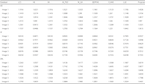
Table 9Fitness value comparison between results obtained using different enhancement methods on standard benchmark face

datasets

AR

Image 1 1.1916 1.0221 1.1916 1.3521 1.3325 1.1961 1.3123 1.1785 1.4028

Image 2 1.1419 1.0174 1.1419 1.3008 1.299 1.1939 1.267 1.1148 1.3154

Image 3 1.2341 1.0914 1.2341 1.3846 1.3868 1.2357 1.3731 1.1828 1.4817

Image 4 1.2572 1.009 1.2572 1.3702 1.3653 1.3082 1.326 1.1349 1.497

Image 5 1.2301 0.9413 1.2301 1.3332 1.3325 1.2836 1.3289 1.1459 1.5531

Image 6 1.1537 0.9486 1.1537 1.2783 1.2784 1.1364 1.223 1.0442 1.3613

YF

Image 1 0.8143 0.6871 0.8143 0.8565 0.8484 0.8464 0.8161 0.7945 0.9337

Image 2 0.9362 0.7971 0.9362 0.9269 0.9316 0.9021 0.8644 0.7126 1.0098

Image 3 0.9501 0.7014 0.9501 0.8319 0.7145 0.9362 0.8546 0.7474 0.9629

Image 4 1.0383 0.8859 1.0383 0.9645 0.9625 0.8961 0.9274 0.7701 1.0682

Image 5 0.8376 0.5986 0.8376 0.5746 0.5739 0.7746 0.7293 0.6559 0.7012

Image 6 0.8234 0.5937 0.8234 0.7194 0.5956 0.8285 0.7416 0.6598 0.7355

ORL

Image 1 1.2263 1.0357 1.2263 1.4126 1.4177 1.2354 1.3308 1.1807 1.6019

Image 2 1.4101 1.2308 1.4101 1.7742 1.7743 1.4209 1.6695 1.4297 1.9877

Image 3 1.3859 1.2339 1.3859 1.6243 1.6227 1.3896 1.5657 1.4284 1.8498

Image 4 1.3368 1.1461 1.3368 1.5423 1.5061 1.3421 1.5291 1.3491 1.8439

Image 5 1.3324 1.3522 1.3324 1.6258 1.6303 1.3604 1.4815 1.3611 1.7788

(13)

improve on the original images, thereby revealing more information in the image.

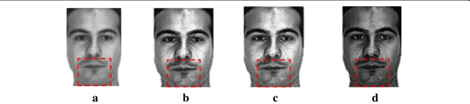
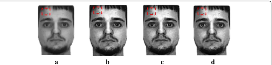
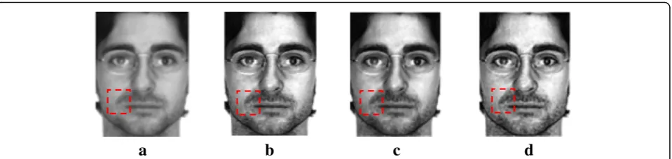
To confirm our selection of the CSO metaheuristic al-gorithm, we qualitatively analyzed the enhanced images produced by the different metaheuristic algorithms with the proposed EF as shown in Figs. 3, 4, and 5. We inserted red bounding boxes in Figs. 3, 4, 5, 6, 7, and8

to emphasize particular regions of interest. For example, observe the bounding box in the original image of Fig.3

and notice that the beards of the subject are significantly revealed in the subsequent enhanced images (see Fig.3b, c, and d). We applied our method based on different metaheuristic algorithms and showed qualitatively (see Figs. 3, 4, and5) that there is not much to differentiate between these optimization algorithms by qualitative analysis. However, we showed slight advantages of the CSO algorithm over other methods by the quantitative results presented in Table2. Furthermore, consider Fig.4

and observe that the four spots within the bounding box in the original image are unobvious; however, they are clearly enhanced and made visible in the enhanced im-ages (see Fig.4b, c, and d). Similarly, we show bounding boxes on other images to emphasize interesting features that have been clearly enhanced over the respective ori-ginal images. In essence, the CSO algorithm provided better quantitative performance as compared to the PSO and GA algorithms.

4.3 Comparison of different EFs

In this section, we confirm the performance of our pro-posed EF based on the CSO algorithm. Hence, we compared the different EFs used in Munteanu [5] and Ye [13] using the CSO algorithm based on three differ-ent selected face images that vary among individuals as shown in Table3.

Considering Table3, the different EFs were compared based on all the performance evaluation metrics using the CSO algorithm. The results obtained confirm the ef-fectiveness of our proposed EF by displaying decent re-sults reported as follows: across images 1, 2, and 3, our proposed EF produced the highest foreground value of 2104, 1116, and 4827, respectively as compared to the other EFs. Similarly, values generated for the number of edges by our proposed algorithms outperformed other EF techniques with higher values of 2304, 2057, and 3368 for images 1, 2, and 3, respectively. Furthermore, the fitness value generated by the different algorithms was analyzed, and it showed that our proposed algorithm produced the highest fitness value for all the images.

To confirm the effectiveness of our proposed EF, a comparison of the different EFs was conducted by ana-lyzing qualitatively the enhanced images as shown in

Figs. 6, 7, and 8. Following these figures, it is evident that our proposed EF outperforms the other algorithms.

4.4 Comparison of different image enhancement methods

The experiments in this section were designed to con-firm the performance of our proposed algorithm by comparing our method with other state-of-the-art image enhancement methods. The methods considered are the linear contrast stretching (LCS), histogram equalization (HE), image intensity adjustment (IIA), Munteanu with particle swarm optimization (M_PSO), Munteanu with genetic algorithm (M_GA), brightness preserving dy-namic fuzzy histogram equalization (BPDFHE), contrast limited adaptive histogram equalization (CLAHE), and low-light image enhancement (LLIE). The results ob-tained are presented in Tables 4, 5, 6, 7, 8, and 9. We conducted these experiments using different standard benchmark face datasets by selecting six different face images with different real-world conditions. The chosen face images selected from each face dataset were labeled images 1–6, and they represent multiple faces with lightning conditions, pose variations, and facial expres-sions such as smile, anger, scream, left light, right light, and both light on, respectively.

From Table 4, the performance of the different image enhancement methods was analyzed based on the num-ber of pixels in the foreground, which represents the amount of information introduced to the enhanced image. Hence, the goal is to obtain a higher number of pixels in the foreground. Our proposed algorithm pro-duced the highest number of pixels in the foreground value across all images within the different face datasets. For image 1 from the AR face dataset, the number of pixels in the foreground value was 3294 achieved by our method, followed by the M_PSO with a value of 2565, then M_GA with a value of 2249, and LCS with a value of 451. Our enhancement method produced for im-ages 2–6 the following number of pixels in the fore-ground values: 2565, 5424, 5956, 6865, and 3947, respectively, which surpasses the values presented by other enhancement methods. For the YF face dataset, our method produced a significant number of pixel values in the foreground across all face images. Similarly, for the ORL face dataset, our method produced the lar-gest number of pixels in the foreground based on the different selected face images. Using this dataset, the values produced for images 1–6 include 10,483, 3873, 7618, 6499, 6248, 5946, and 4705, respectively.

(14)

edges because it demonstrates that more information has been added to the enhanced image. M_GA follows with the largest number of edge values across all images, while LCS and BPDFHE produced the least number of edge values.

Tables 6, 7, and 8 display the PSNR value, entropic measure value, and the AMBE value, respectively. The PSNR value obtained with our method produced the lowest value across all face images within the different face datasets. This implies that a lower PSNR value pro-duces a more enhanced image. The entropic value by our proposed technique produced a higher value for most face images as compared to the other methods. This shows that more information has been added to the enhanced image to make the face image unique. Further,

the AMBE values of each method, representing the mean brightness value, were compared. Our method preserved the absolute mean brightness error value sig-nificantly. Furthermore, the fitness values of each method were computed and presented in Table 9. The fitness value is an important metric that determines the effectiveness of each technique, and a higher fitness value is desired. Our method when compared to the other IETs produced the highest fitness value across most face images used from the different face datasets. Our method is followed by the M_PSO method across all images. The CLAHE and BPDFHE methods produced a satisfactory performance while the HE method produced the least fitness value across all images.

Fig. 9Qualitative comparison of the different image enhancement algorithms on the AR face dataset where Figs.1,2,3,4,5, and6represent

images of different subjects respectively.a–jdenote the methods labeled asaoriginal,bLCC,cHE,dIIA,eM_PSO,fM_GA,gBDPFHE,hCLAHE,

(15)

To confirm further the performance of our proposed algorithm, we compared qualitatively the enhanced im-ages produced by the different image enhancement methods as shown in Figs.9,10, and11with each figure representing different lightning conditions, pose vari-ation, and facial expressions such as smile, anger, scream, left light on, right light on, and both light on, respectively.

Figures 9, 10, and 11 display the effectiveness of our proposed IETs. The enhanced images produced by our

algorithm show a much positive difference in quality than the original and other enhanced images by other methods. The images affected by lighting conditions, i.e., images 4, 5, and 6 representing right light, left light and both light on, respectively were effectively enhanced as compared to other enhancement techniques. Further-more, our method produced decent enhanced images considering images with different pose and expressions. Generally, unlike the images produced by other methods, our method produced more enhanced face

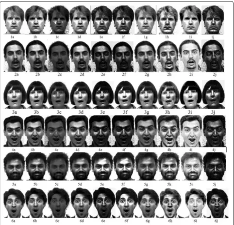
Fig. 10Qualitative comparison of the different image enhancement algorithms on the Yale face dataset where Figs.1,2,3,4,5, and6represent

images of different subjects respectively. anda–jdenote the methods labeled asaoriginal,bLCC,cHE,dIIA,eM_PSO,fM_GA,gBDPFHE,h

(16)

images. This better performance was achieved because our method considers different essential metrics in its design. Metrics such as the number of edges and the number of the pixel value in the foreground will un-doubtedly add more features to the image, thus, produ-cing a more enhanced image.

4.5 Processing time per image

In this section, we provide results concerning the pro-cessing time of each algorithm per image considered in our research. We conducted the experiments in this sec-tion using a PC built on an Intel Core i5 processor with an Intel HD Graphics 4400 and 8GB RAM. We tested

Fig. 11Qualitative comparison of the different image enhancement algorithms on the ORL face dataset where Figs.1,2,3,4,5, and6represent

images of different subjects respectively.a–jdenote the methods labeled asaoriginal,bLCC,cHE,dIIA,eM_PSO,fM_GA,gBDPFHE,hCLAHE,

iLLIE, andjproposed

Table 10Processing time per facial image comparison using the different image enhancement methods on different image pixel

size

Image pixel Methods

LCS HE IIA M_PSO M_GA BDPFHE CLAHE LLIE Proposed

64 × 64 0.115 0.117 0.114 3.635 3.783 0.114 0.133 0.202 11.155

128 × 128 0.144 0.145 0.143 13.736 14.0451 0.140 0.151 0.231 27.363

(17)

each algorithm using three different pixel sizes in order to assess their respective average processing times. The results obtained are presented in Table 10. Our algo-rithm experienced the longest average processing time per image. The processing time increased as the image pixel size increased. Our method experienced a longer processing delay because it computes iteratively both in the transformation and in the evaluation blocks for each potentially enhanced image in a population of several solutions. This iteration in the optimization process further prolonged the processing time of our method. This indicates that a trade-off thus exists between achieving better-enhanced images at the ex-pense of speed. Though our method experienced a longer delay than other alternatives; however, this delay was at a far better enhancement performance than the other alternatives. Practical application areas where our method can be applied are as follows: in face enhancement and editing software in smart-phones, face enhancement for forensic purposes, and face enhancement for cosmetic and dermatological purposes. In these and other similar application areas, experts are notably interested more in better-enhanced images than in the speed of enhancement. Nevertheless, we have observed that metaheuristic-based methods tend to provide improved performance than other methods at the expense of longer process-ing times.

5 Conclusion

Image enhancement is an essential pre-processing stage in typical face recognition systems. Hence, an efficient IET is required in order to improve face recognition per-formance. In this paper, we have presented a new EF for face image enhancement in unconstrained environments using metaheuristic algorithms. Our EF is used in conjunction with the cuckoo search optimization (CSO) algorithm to determine the best enhanced image, similar to the visual role played by a human evaluator. We achieved improved performance by introducing a scaled mechanism in our EF that prevents the enhanced image from assuming extreme dark or bright images. We have shown that our proposed EF outperforms other stand-ard EFs. In addition, extensive quantitative and quali-tative comparisons with other metaheuristic and state-of-the-art image enhancement methods were conducted in order to demonstrate the effectiveness of our method. We evaluated our method using dif-ferent face images from difdif-ferent standard benchmark face datasets that represent different real-life scenar-ios. The performance metrics considered in our re-search demonstrated the superior performance of our method over other methods. For future works, we will look at the possibility of exploring other metaheuristic

algorithms. In addition, approaches to reduce the processing time per image using the proposed method will be investigated. We note that our work can be extended to other application areas of image process-ing in order to improve their respective performance rates.

Abbreviations

AHE:Adaptive histogram equalization; AMBE: Absolute mean brightness error; BPDFHE: Brightness preserving dynamic fuzzy histogram equalization; CSO: Cuckoo search optimization; EF: Evaluation function; GA: Genetic algorithm; HE: Histogram equalization; IET: Image enhancement technique; IIA: Image intensity adjustment; LCS: Linear contrast stretching; LLIE: Low-light image enhancement; PSNR: Peak signal-to-noise ratio; PSO: Particle swarm optimization

Acknowledgements

The authors will like to thank the editor, associate editor and peer reviewers for all their comments.

Funding

This work was supported by the Council for Scientific and Industrial Research (CSIR), South Africa. [ICT: Meraka].

Availability of data and materials

The AR, Yale and ORL face datasets were used to confirm our proposed methods.

Authors’contributions

MO was the main contributor to the design of the new image enhancement algorithm and drafted the manuscript. GH and HM edited and modified the overall content of the manuscript while also giving adequate supervision. AO participated in the discussion of this work. All authors read and approved the final manuscript.

Competing interests

The authors declare that they have no competing interests.

Publisher’s Note

Springer Nature remains neutral with regard to jurisdictional claims in published maps and institutional affiliations.

Received: 1 August 2018 Accepted: 9 January 2019

References

1. M.O. Oloyede, G.P. Hancke, Unimodal and multimodal biometric sensing systems: a review. IEEE Access4, 7532–7555 (2016)

2. Z. Shi, M. mei Zhu, B. Guo, M. Zhao, C. Zhang, Nighttime low illumination image enhancement with single image using bright/dark channel prior. EURASIP J. Image Video Proc.2018(1), 13 (2018)

3. N. Dagnes, E. Vezzetti, F. Marcolin, S. Tornincasa, Occlusion detection and restoration techniques for 3D face recognition: a literature review. Mach Vis Appl29, 789–813 (2018)

4. M. Sharif, M.A. Khan, T. Akram, M.Y. Javed, T. Saba, A. Rehman, A framework of human detection and action recognition based on uniform

segmentation and combination of Euclidean distance and joint entropy-based features selection. EURASIP J. Image Video Proc.2017(1), 89 (2017) 5. C. Munteanu, A. Rosa, Gray-scale image enhancement as an automatic

process driven by evolution. IEEE Trans. Syst. Man Cybern. Part B (Cybernetics)34(2), 1292–1298 (2004)

6. H.-T. Wu, S. Tang, J.-L. Dugelay, Image reversible visual transformation based on MSB replacement and histogram bin mapping. in Proceedings of the IEEE Tenth International Conference on Advanced Computational Intelligence (ICACI) Xiamen, 813–818 (2018)

(18)

8. K. Hussain et al., A histogram specification technique for dark image enhancement using a local transformation method. IPSJ Trans. Comput. Vision Appl.10(1), 3 (2018)

9. B.-V. Le, S. Lee, T. Le-Tien, Y. Yoon, Using weighted dynamic range for histogram equalization to improve the image contrast. EURASIP J. Image Video Proc.2014(1), 44 (2014)

10. Y. Cheng, L. Jiao, X. Cao, Z. Li, Illumination-insensitive features for face recognition. Vis. Comput.33(11), 1483–1493 (2017)

11. J.R. Tang, N.A.M. Isa, Bi-histogram equalization using modified histogram bins. Appl. Soft Comput.55, 31_–43 (2017)

12. M. Barni, E. Nowroozi, B. Tondi, inProceeding of the IEEE International Workshop on Biometrics and Forensics (IWBF), Sassari. Detection of adaptive histogram equalization robust against JPEG compression (2018), pp. 1–8 13. Z. Ye, M. Wang, Z. Hu, W. Liu, An adaptive image enhancement technique

by combining cuckoo search and particle swarm optimization algorithm. Comput Intell Neurosci2015, 13 (2015)

14. P.B. Aquino-Morínigo, F.R. Lugo-Solís, D.P. Pinto-Roa, H.L. Ayala, J.L.V. Noguera, Bi-histogram equalization using two plateau limits. SIViP11(5), 857_–864 (2017) 15. X. Wang, L. Chen, Contrast enhancement using feature-preserving

bi-histogram equalization. Signal Image and Video Processing,12(4), 1–8 (2017) 16. K. Singh, R. Kapoor, Image enhancement using exposure based sub image

histogram equalization. Pattern Recogn. Lett.36, 10_–14 (2014)

17. L. Zhuang, Y. Guan, Image enhancement via subimage histogram equalization based on mean and variance. Comput Intell Neurosci2017, 1–12 (2017) 18. A. Mustapha, A. Oulefki, M. Bengherabi, E. Boutellaa, M.A. Algaet, Towards

nonuniform illumination face enhancement via adaptive contrast stretching. Multimed. Tools Appl.76(21), 21961–21999 (2017)

19. K. Hasikin, N.A.M. Isa, Adaptive fuzzy contrast factor enhancement technique for low contrast and nonuniform illumination images. SIViP8(8), 1591–1603 (2014) 20. S. Rahman, M.M. Rahman, M. Abdullah-Al-Wadud, G.D. Al-Quaderi, M.

Shoyaib, An adaptive gamma correction for image enhancement. EURASIP J. Image Video Proc.2016(1), 35 (2016)

21. K.G. Dhal, S. Das, Cuckoo search with search strategies and proper objective function for brightness preserving image enhancement. Pattern Recog. Image Anal.27(4), 695–712 (2017)

22. J.-B. Martens, L. Meesters, Image dissimilarity. Signal Process.70(3), 155–176 (1998) 23. A. Bhandari, A. Kumar, S. Chaudhary, G. Singh, A new beta differential

evolution algorithm for edge preserved colored satellite image enhancement. Multidim. Syst. Sign. Process.28(2), 495–527 (2017) 24. M. Abdel-Basset, A.-N. Hessin, L. Abdel-Fatah, A comprehensive study of

cuckoo-inspired algorithms. Neural Comput. Applic.29(2), 345–361 (2018) 25. W. Xi, T. Wu, K. Yan, X. Yang, X. Jiang, N. Kwok, Restoration of online video ferrography images for out-of-focus degradations. EURASIP J. Image Video Proc.2018(1), 31 (2018)

26. J.-P. Pelteret, B. Walter, P. Steinmann, Application of metaheuristic algorithms to the identification of nonlinear magneto-viscoelastic constitutive parameters. J. Magn. Magn. Mater.464, 116 (2018)

27. X.-S. Yang and S. Deb,“Cuckoo search via Lévy flights,”in Proceeding of the IEEE World Congress on Nature & Biologically Inspired Computing, NaBIC Coimbatore 2009, pp. 210_–214

28. B. Yang, J. Miao, Z. Fan, J. Long, X. Liu, Modified cuckoo search algorithm for the optimal placement of actuators problem. Appl. Soft Comput.67, 48–60 (2018)

29. A.M. Martinez, The AR face database, CVC Technical Report 24 (1998) 30. Z. Krbcova, J. Kukal, Relationship between entropy and SNR changes in

image enhancement. EURASIP J. Image Video Proc.2017(1), 83 (2017) 31. S. Suresh, S. Lal, Modified differential evolution algorithm for contrast and