R E S E A R C H
Open Access
Steganalysis of JSteg algorithm using
hypothesis testing theory
Tong Qiao
*, Florent Retraint, Rémi Cogranne and Cathel Zitzmann
Abstract
This paper investigates the statistical detection of JSteg steganography. The approach is based on a statistical model of discrete cosine transformation (DCT) coefficients challenging the usual assumption that among a subband all the coefficients are independent and identically distributed (i. i. d. ). The hidden information-detection problem is cast in the framework of hypothesis testing theory. In an ideal context where all model parameters are perfectly known, the likelihood ratio test (LRT) is presented, and its performances are theoretically established. The statistical performance of LRT serves as an upper bound for the detection power. For a practical use where the distribution parameters are unknown, by exploring a DCT channel selection, a detector based on estimation of those parameters is designed. The loss of power of the proposed detector compared with the optimal LRT is small, which shows the relevance of the proposed approach.
Keywords: hypothesis testing theory; JSteg steganalysis; DCT distribution model; Hidden information detection
1 Introduction
Steganography and steganalysis have received more and more focus in the past two decades since the research in this field concerns law enforcement and national strate-gic defence. Steganography is the art and science of hiding secret messages in the cover media. On the opposite, steganalysis is about the detection of hidden secret infor-mation embedded in the cover media, also called stego media. If a steganalysis algorithm detects the inspected media as the stego one, even without knowing any extra information about the secret message, the steganographic approach fails.
1.1 State of the art
In today’s digital world, there exists many steganographic tools available on the Internet. Due to the fact that some are readily available and very simple to use, it is neces-sary to design the most reliable steganalysis methodology to fight back steganography. In general, due to its sim-plicity, most steganographic schemes insert the secret message into the least significant bit (LSB) plane of the cover media, including two kinds of steganography: LSB
*Correspondence: [email protected]
ICD - LM2S - Université de Technologie de Troyes (UTT) - UMR STMR CNRS, 12 rue Marie Curie, 10004 Troyes, France
replacement and LSB matching. The former algorithm aims at replacing the LSB plane in the spatial domain or frequency domain of the cover media by 0 or 1. The lat-ter algorithm, also known as ±1 embedding (see [1-3]), randomly increments or decrements a pixel or discrete cosine transformation (DCT) coefficient value to match the secret bit to be embedded when necessary. Since LSB replacement is easier to implement, it remains more pop-ular, and hence, as of December 2011, WetStone declared that about 70% of the available steganographic soft-wares are based on the LSB-replacement algorithm [4]. Therefore, the research on LSB-replacement steganalysis remains an active topic.
Although the LSB-replacement steganalysis method (see [5-10]) has been studied for many years, it can be noted that most of the prior-art detectors are designed to detect data hidden in the spatial domain. In addition, for only a few detectors, the statistical properties have been studied and established, referred to as the optimal detectors. As detailed in [11], a wide range of prob-lems, theoretical as well as practical, remain uncovered and some prevent the moving of ‘steganography and ste-ganalysis from the laboratory into the real world’. This is especially the case in the field of optimal detection, see ([11] , sec. 3.1), in which this paper lies. Roughly speaking, the goal of optimal detection in steganalysis is
to exploit an accurate statistical model of cover source, usually digital images, to design a statistical test whose properties can be established, typically, in order to guar-antee a false alarm rate (FAR) and to calculate the optimal detection performance one can expect from the most powerful detector.
In 2004, the weighted stego-image (WS) method [12] and the test proposed in [13] for LSB-replacement ste-ganalysis changed the situation opening the way to optimal detectors. Driven by these pioneer works, the enhanced WS algorithm proposed in [14] improved the detection rate by enhancing pixel predictor, adjusting weighting factor and introducing the concept of bias cor-rection. Nevertheless, the drawback of the original WS method is that it can only be applied in the spatial domain. Due to the prevalence of images compressed in the Joint Photographic Experts Group (JPEG) format, how to deal with this kind of images becomes mandatory. Inspired by the prior studies [12,14], the WS steganalyser for JPEG covers was proposed in [15]. However, the WS steganal-yser does not allow one to get a high-detection perfor-mance for a low FAR, see [16], and its statistical properties remain unknown, which prevents the guarantee of a pre-scribed FAR. In practical forensic cases, since a large database of images needs to be processed, the getting of a very low FAR is crucial.
1.2 Contributions of the paper
For the detection of data hidden within the DCT coef-ficients of JPEG images, the application of hypothesis testing theory for designing optimal detectors that are efficient in practice is facing the problem of accurately modelling statistical distribution of DCT coefficients. It can be noted that several models have been proposed in the literature to model statistically the DCT coefficients. Among those models, the Laplacian distribution is prob-ably the most widely used due to its simplicity and its fairly good accuracy [17]. More accurate models such as the generalized Gaussian [18] and, more recently, the gen-eralized gamma model [19] have been shown to provide much more accuracy at the cost of higher complexity. Some of those models have been exploited in the field of steganalysis, see [20,21] for instance. In the framework of optimal detection, a first attempt has been made to design a statistical test modelling the DCT coefficient with the quantized Laplacian distribution, see [22].
It should be noted that other approaches have been proposed for the detection of data hidden within DCT coefficients of JPEG images, to cite a few, the structural detection [23], the category attack [24], the WS detec-tor [15] and the universal or blind detecdetec-tors [25,26]. However, establishing the statistical properties of those detectors remains a difficult work which has not been studied yet. In addition, most accurate detectors based
on statistical learning are sensitive to the so-called cover-source mismatch [27]: the training phase must be per-formed with caution.
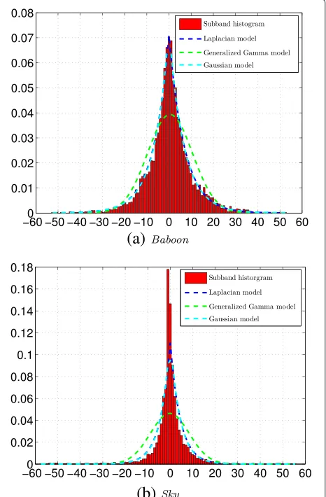
In this context, the detector proposed in [22] is an inter-esting alternative; however, it is based on the assumption that DCT coefficients are independent and identically distributed (i. i. d. ) within a subband and have a zero expectation which might be inaccurate and hence make the detection performance poor in practice. In practice, this model is not independent of the image content, which performs well only in the case of a high-texture image (see Figure 1a), but hardly holds true in the case of a low-texture image (see Figure 1b). On the opposite, this paper proposes a statistical model assuming that each DCT coefficient has a different expectation and variance. The use of this model, together with hypothesis theory, allows us to design the most powerful likelihood ratio test (LRT) when the distribution parameters (expectation and variance) are known. Then, in the practical case of not
(a)
(b)
knowing those parameters, estimations have to be used instead; this leads to the design of the proposed detector with estimated parameters. By taking into account those distribution parameters as nuisance parameters and using an accurate estimation, it is shown that the loss of power compared with the optimal detector is small.
Therefore, the contributions of this paper are as follows:
1. First, a novel model of DCT coefficients is proposed; its major originality is that this model does not assume that all the coefficients of the same subband are i. i. d.
2. Second, assuming that all the parameters are known, this statistical model of DCT coefficients is used to design the optimal test to detect data hidden within JPEG images with JSteg algorithm. This statistical test takes into account distribution parameters of each DCT coefficient as nuisance parameters. 3. Further, assuming that all the parameters are
unknown, a simple approach is proposed to estimate the expectation (or location) parameter of each coefficient by using linear properties of DCT as well as estimation of pixel expectation in the spatial domain; the variance (or scale) parameter is also estimated locally.
4. The designed detector is improved by exploring a DCT channel selection, which has been proposed very recently [28,29] that selects only a subset of pixels or DCT coefficients in which embedding is most likely and hence detection easier.
5. Numerical results show the sharpness of the theoretically established results and the good performance of the proposed statistical test. A comparison with the statistical test based on the Laplacian distribution and on the assumption of i. i. d. coefficient, see [22], shows the relevance of the proposed methodology. In addition, compared with prior-art WS detector [15], experimental results show the efficiency of the proposed detector.
1.3 Organisation of the paper
This paper is organised as follows. Section 2 formalises the statistical problem of detection of information hidden within DCT coefficients of JPEG images. Then, Section 3 presents the optimal LRT for detecting the JSteg algorithm based on the Laplacian distribution model. Section 4 presents the proposed approach for estimating the nui-sance parameters in practice and compares our proposed detector with the WS detector [15] theoretically. Finally, Section 5 presents numerical results of the proposed ste-ganalyser on simulated and real images, and Section 6 concludes this paper. This paper is an extended version of [30] that also includes the findings of [31] on channel selection [28,29].
2 Problem statement
In this paper, a grayscale digital image is represented, in the spatial domain, by a single matrix Z = {zi,j},i ∈ {1,. . .,I},j ∈ {1,. . .,J}. The present work can be extended to a colour image by analysing each colour chan-nel separately. Most digital images are stored using the JPEG compression standard. This standard exploits the linear DCT, over blocks of 8 × 8 pixels, to represent an image in the so-called DCT domain. In the present paper, we avoid the description of the imaging pipeline of a digital still camera; the reader can refer to [32] for a description of the whole imaging pipeline and to [33] for a detailed description of the JPEG compression standard.
Let us denote DCT coefficients by the matrix V =
{vi,j}. An alternative representation of those coefficients is usually adopted by gathering the DCT coefficients that correspond to the same frequency subband. In this paper, this alternative representation is denoted by the matrix U = {uk,l},k ∈ {1,. . .,K},l ∈ {1,. . ., 64} with K ≈ I×J/64a.
The coefficients from the first subband uk,1, often
referred to as direct current component (DC) coefficients, represent the mean of pixel value over a k-th block of 8×8 pixels. The modification of those coefficients may be obvious and creates artifacts that can be detected easily; hence, they are usually not used for data hiding. Similarly, the JSteg algorithm does not use the coefficients from the other subbands, referred to as alternating current compo-nent (AC) coefficients, if they equal 0 or 1. In fact, it is known that using the coefficients equal to 0 or 1 modifies significantly the statistical properties of AC coefficients; this creates a flaw that can be detected.
The JSteg algorithm embeds data within the DCT coefficients of JPEG images using the well-known LSB-replacement method, see details in [34]. In brief, this method consists of substituting the LSB of each DCT coefficient by a bit of the message it is aimed to hide. The number of bits hidden per coefficient, usually referred to as the payload, is denotedR∈(0, 1]. Since the JSteg algo-rithm does not use each DCT coefficient, the payload will in fact be measured in this paper as the number of bits hidden perusablecoefficients (that is the number of bits divided by the number of AC coefficients that differ from 0 and 1).
R. A short calculation shows that, see [8,12,13], the stego-image distribution may be represented by following the pmfQRθ =qθR[u]u∈Zwhere:
qRθ[u]=(1−R/2)pθ[u]+R/2pθ[u¯] , (1) andu¯ = u+(−1)urepresents the integeruwith flipped LSB. For the sake of clarity, let us denoteθk,l the distri-bution parameter of the k-th DCT coefficient from the
l-th subband and let θ = {θk,l},k ∈ {1,. . .,K},l ∈ {2,. . ., 64}represent the distribution parameter of all the AC coefficients.
When inspecting a given JPEG image, more precisely its DCT coefficients matrix U, in order to detect data hidden with the JSteg algorithm, the problem consists in choosing between the two following hypotheses:H0: ‘the
coefficientsuk,lfollow the distributionPθk,l’ andH1: ‘the coefficientsuk,lfollow the distributionQRθk,l’ which can be written formally as:
⎧ ⎨ ⎩
H0:
uk,l∼Pθk,l,∀k∈ {1,. . .,K},∀l∈ {2,. . ., 64}
,
H1:
uk,l∼QRθk,l,∀k∈ {1,. . .,K},∀l∈ {2,. . ., 64}
.
(2)
A statistical test is mappingδ : ZI·J → {H0,H1} such
that hypothesis Hi is accepted if δ(U) = Hi (see [35] for details on hypothesis testing). As previously explained, this paper focuses on the Neyman-Pearson bi-criteria approach: maximising the correct detection probability for a given false alarm probabilityα0. Let:
Kα0 = δ: sup
θ PH0[δ(U)=H1]≤α0
, (3)
be the class of tests with a false alarm probability upper bounded by α0. Here, PHi(A) stands for the probabil-ity of event A under hypothesisHi,i = {0, 1}, and the supremum overθ has to be understood as whatever the distribution parameters might be, in order to ensure that the false alarm probabilityα0cannot be exceeded. Among all the tests inKα0, it is aimed at finding a testδ which maximises the power function, defined by the correct detection probability:
βδ=PH1[δ(U)=H1] , (4)
which is equivalent to minimise the missed detection probabilityα1(δ)=PH1[δ(U)=H0]=1−βδ.
In order to design a practical optimal detector, as referred in [11], for steganalysis in the spatial domain, the main difficulty is to estimate the distribution parameters (expectation and variance of each pixel). On the oppo-site, in the case of the DCT coefficients, the application of hypothesis testing theory to design an optimal detector has previously been attempted with the assumption that
the distribution parameter remains the same for all the coefficients from a same subband. With this assumption, the estimation of the distribution parameters is not an issue because thousands of DCT coefficients are available. However, which distribution model to choose remains an open problem.
The hypothesis testing theory has been applied for the steganalysis of JSteg algorithm in [22] using a Laplacian distribution model and using the assumption that DCT coefficients of each subband are i. i. d. However, this pio-neer work does not allow the designing of an efficient test because a very important loss of performance has been observed when comparing results on real images and theoretically established ones. Such a result can be explained by the two following reasons: 1) the Laplacian model might be not accurate enough to detect steganag-raphy and 2) the assumption that the DCT coefficients of each frequency subband are i. i. d. may be wrong. Recently, it has been shown that the use of the generalised gamma model or an even more accurate model [36,37] allows the designing of a test with very good detection per-formance. On the opposite, in this paper, it is proposed to challenge the assumption that all the DCT coefficients of a subband are i. i. d.
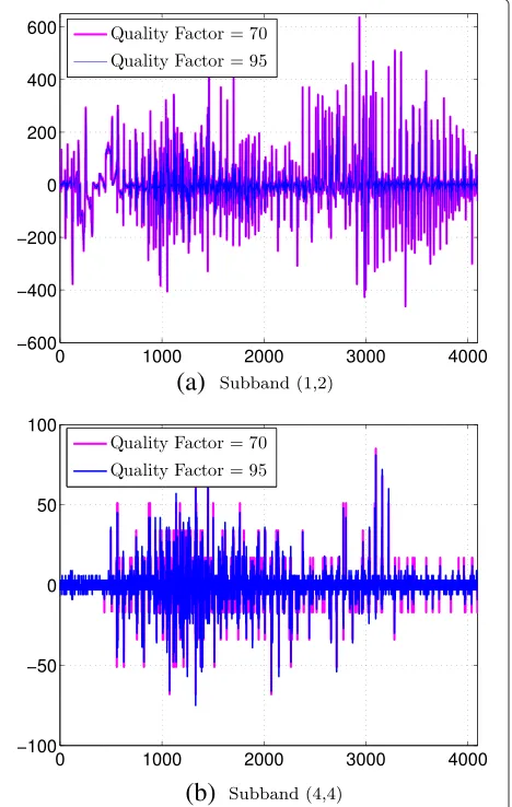
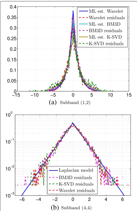
A typical example is given by Figures 2 and 3. Figure 2a and Figure 2b, respectively, represent the DCT coeffi-cients of the subband (1,2) and subband (4,4) extracted from the image lena. Observing those two graphs, it is obvious that the assumption of all those coefficients being i. i. d. is doubtful. However, if it is assumed that each coefficient has a different expectation, one can estimate this expected value and compute the ‘residual noise’, that is, the difference between the observation and the com-puted expectation. Such results are shown in Figure 3, with three different models for estimating the expectation of DCT coefficients of the same two subbands fromlena. Moreover, Figure 4 illustrates the distribution of residual noises which are plotted in Figure 3. Obviously, resid-ual noises look much more i. i. d. than the original DCT coefficients.
In the following section, we detail the statistical test that takes into account both the expectation and the variance as nuisance parameters, and we study the optimal detec-tion when those parameters are known. A discussion on nuisance parameters is also provided in Section 4.
3 LRT for two simple hypothesis
3.1 Optimal detection framework
When the payload R and the distribution parameters
(a)
(b)
Figure 2Illustrative examples of the value of DCT coefficients of two subbands (a, b) from thelenaimage.Those examples show that the assumption that DCT coefficients are i. i. d. within a subband hardly holds true in practice.
the assumption that DCT coefficients are independent, as:
δlr(U)= ⎧ ⎪ ⎪ ⎪ ⎪ ⎪ ⎨ ⎪ ⎪ ⎪ ⎪ ⎪ ⎩
H0iflr(U)= K
k=1 64
l=2 lr(u
k,l) < τlr,
H1iflr(U)= K
k=1 64
l=2 lr(u
k,l)≥τlr, (5)
where the decision threshold τlr is the solution of the equationPH0lr(U)≥τlr=α0, to ensure that the false alarm probability of the LRT equalsα0, and the log likeli-hood ratio (LR) for one observation is given, by definition, by:
lr(u
k,l)=log
qRθ k,l[uk,l] pθk,l[uk,l]
. (6)
(a)
(b)
Figure 3Illustrative examples of DCT coefficients of residual noise, obtained by denoising image.The same two DCT subbands (a, b), as in Figure 2 are extracted the residual noise oflenaimage. On those examples, the assumption of i.i.d. distribution seems to be more realistic. It is noted that three denoising filters are respectively designed based on wavelet, block-matching and 3D (BM3D) and dictionary learning (K-SVD) algorithms.
In practice, when the rateRis not known, one can try to design a test which is locally optimal around a given pay-load rate, named Locally Asymptotically Uniformly Most Powerful (LAUMP) test, as proposed in [6,8], but this lies outside the scope of this paper.
From the definition ofpθk,l[uk,l] andqRθk,l[uk,l] (1), it is easy to write the LR (6) as:
lr(u
k,l)=log
1−R 2 +
R
2
pθk,l[u¯k,l]
pθk,l[uk,l]
, (7)
(a)
(b)
Figure 4Statistical distribution of the DCT coefficients of the residual noise plotted in Figure 3.For comparison, the Laplacian pdf with parameters estimated by the maximum likelihood estimation (ML est.) are also shown in(a). Note that for a meaningful comparison,(b)shows the results after normalization by the estimated scale parameterbk. It is noted that three denoising filter are
respectively designed based on wavelet, block-matching and 3D (BM3D) and dictionary learning (K-SVD) algorithms.
3.2 Statistical performance of LRT
Accepting, for a moment, that one is in this most favourable scenario, in which all the parameters are per-fectly known, we can deduce some interesting results. Due to the fact that observations are considered to be indepen-dent, the LRlr(U)is the sum of random variables and some asymptotic theorems allow to establish its distribu-tion when the number of coefficients becomes ‘sufficiently large’. This asymptotic approach is usually verified in the case of digital images due to the very large number of pixels or DCT coefficients.
Let us denote EHi(θk,l) and VHi(θk,l) the expectation and the variance, respectively, of the LRlr(uk,l) under hypothesis Hi,i = {0, 1}. Those quantity obviously
depend on the parameterized distribution Pθk,l. The Lindeberg’s central limit theorem (CLT) ([35], theorem 11.2.5) states that asKtends to infinity it holds true thatc:
K
k=1 64
l=2 lr(u
k,l)−EHi(θk,l) K
k=1 64
l=2
VHi(θk,l) 1/2
d
−→N(0, 1),i= {0, 1},
(8)
where−→d represents the convergence in distribution, and N(0, 1)is the standard normal distribution, i.e. with zero mean and unit variance.
This theorem is of crucial interest to establish the sta-tistical properties of the proposed test [7,22,37,38]. In fact, once the moments have been calculated under both Hi,i= {0, 1}, one can normalise under hypothesisH0the
LRlr(U)as follows:
lr(U)=
lr(U)−K k=1
64
l=2EH0(θk,l)
K
k=1 64
l=2VH0(θk,l)
1/2 ,
= K
k=1 64
l=2lr(uk,l)−EH0(θk,l)
K
k=1 64
l=2VH0(θk,l)
1/2 .
(9)
Since this essentially consists of adding a deterministic value and scaling the LR, this operation of normalisation preserves the optimality of the LRT. It is thus straightfor-ward to define the normalised LRT withlr(U)by:
δlr(U)= ⎧ ⎨ ⎩
H0if lr(U) < τlr
H1if lr(U)≥τlr.
(10)
It immediately follows from Lindeberg’s CLT (8) that
lr(U)asymptotically follows, asK tends to infinity, the normal distributionN(0, 1). Hence, it is immediate to set the decision threshold that guarantees the prescribed false alarm probability:
τlr=−1(1−α0), (11)
where and −1, respectively, represent the cumula-tive distribution function (cdf ) of the standard normal distribution and its inverse. Similarly, denoting:
mi= K
k=1 64
l=2
EHi(θk,l);σi2= K
k=1 64
l=2
VHi(θk,l),i={0, 1},
it is also straightforward to establish the detection func-tion of the LRT given by:
βδlr=1−
σ0
σ1−1(1−α0)+
m0−m1 σ1
Equations (11) and (12) emphasise the main advantage of normalising the LR as described in relation (9): it allows setting any threshold that guarantees a false alarm prob-ability independently from any distribution parameters, and, this is particularly crucial because digital images are heterogeneous, their properties vary for each image. Sec-ond, the normalisation allows to easily establish the detec-tion power which again is achieved for any distribudetec-tion parameters and hence for any inspected image.
3.3 Application with Laplacian distribution
In the case of Laplacian distribution, the framework of hypothesis testing theory has been applied for the ste-ganalysis of JSteg in [22] in which the moments of LR are calculated under the two following assumptions: 1) all the DCT coefficients from the same subband are i. i. d. and 2) the expectation of each DCT coefficient is zero.
The continuous Laplacian distribution has the following probability density function (pdf ):
fμ,b(x)= 1 2bexp
−|x−μ| b
(13)
where μ ∈ R, sometimes referred to as the location parameter, corresponds to the expectation, andb > 0 is the so-called scale parameter. During the compression of JPEG images, the DCT coefficients are quantized. Hence, let us define the discrete Laplacian distribution by the following pmf, see details in Appendix A:
fμ,b[k]def=.P
x∈[(k−1/2),(k+1/2)[
= ⎧ ⎨ ⎩
exp−|kb−μ|sinh2b if μ∈/[k−1/2;k+1/2[
1−exp−2bcosh
−(k)−μ
2b
otherwise (14)
whereis the quantization step.
From the expression of the discrete Laplacian distri-bution (14) and from the expression of LR (7), one can express the LR for the detection of JSteg under the assumption that DCT coefficients follow a Laplacian dis-tribution, as follows (see Appendix B):
lr
μ,b[k]=log
1−R 2+
R
2exp
bsign(k−μ)(k− ¯k)
,
(15)
where the observed DCT coefficient, referred to asuk,l in Equation (7), is denoted as k. It can be noted that this expression (15) of the LR is almost the same as the one obtained in [22]; assuming that all DCT coeffi-cients have a zero mean, only the sign term sign(k−μ) becomes sign(k) when assuming a zero mean. It should also be noted that the log-LR equals 0 for every DCT
coefficient whose value is 0 or 1 because the JSteg algo-rithm does not embed hidden data in those coefficients. In the present paper, the moments of the LR (15) are not analytically established; the interested reader can refer to [22].
4 Proposed approach for estimating the nuisance
parameters in practice
4.1 Estimation of expectation of each DCT coefficient As already explained, most statistical models of DCT coef-ficients assume that within a subband the coefcoef-ficients are i. i. d. However, as illustrated in Figures 1 and 2, this assumption is doubtful in practice. Another way to explain why the DCT coefficients may not be i. i. d. is to consider a block of 8×8 pixels in the spatial domain, say the first, z = zi,j,i ∈ {1,. . ., 8},j ∈ {1,. . ., 8}. The value of those pixels can be decomposed as:
zi,j=xi,j+ni,j,
where xi,j is a deterministic value that represents the expectation of a pixel at location (i,j) and ni,j is the realisation of a random variable representing all noises corrupting the inspected image. Clearly, this decomposi-tion can be done for the whole blockz = x+n, where x= {xi,j}andn= {ni,j}. Since the DCT transformation is linear, the DCT coefficient of any block may be expressed as :
DCT(z)=DTzD=DT(x+n)D
=DTxD+DTnD=DCT(x)+DCT(n), (16)
where DCT represents the DCT transform andDis the change of basis matrix from spatial to DCT basis, often referred as the DCT matrix.
It makes sense to assume that the expectation of the noise componentnhas a zero mean in the spatial and in the DCT domain. On the opposite, it is difficult to justify that the DCT of pixels’ expectation x should necessar-ily be around zero. Actually, this assumption holds true if and only if the expectation is the same for of all the pix-els from a block:∀i ∈ {1,. . ., 8},∀j ∈ {1,. . ., 8},xi,j = x; see [36,37,39] for details.
On the opposite, in the paper, it is mainly aimed at estimating the expectation of each DCT coefficient. To this end, it is proposed to decompress a JPEG imageV into the spatial domain to obtainZ, then to estimate the expectation of each pixel in the spatial domainZby using a denoising filter. Then, this denoised imageZis trans-formed back into the DCT domain to finally obtain the estimated value of all DCT coefficients, denoted V =
spatial domain Z, namely, the BM3D collaborative fil-tering [40], K-SVD sparse dictionary learning [41], non-local weighted averaging method from non-non-local (NL) means [42] and the wavelet denoising filter [43]. The codes used for the methods [40-42] have been down-loaded from the Image Processing On-Line websited. The codes used for the method [43] have been downloaded from DDEe.
4.2 A local estimation of b
In addition, the proposed model also assumes that the scale parameterbk,lis different for each DCT coefficient. The estimation of this parameter, for each DCT coeffi-cient, is based on the WS Jpeg method to locally estimate the variance; that is, for coefficientsvi,j, it simply consists of the sample variance of the DCT coefficients of the same subband from neighbouring blocks:
σ2 i,j=
1 7
1
s=−1 1
t=−1
(s,t)=(0,0)
vi+8s,j+8t− ¯vi,j 2
, (17)
wherev¯i,jis the sample mean: 181s=−1 1
t=−1
(s,t)=(0,0)
vi+8s,j+8t. Let
us recall that the MLE of the scale parameter of Lapla-cian distribution from realisationsx1,. . .,xN is given by
ˆ
b=N−1Nn=1|xn−μ|. The local estimation of the scale parameter it is proposed to use in this paper is given by:
ˆ bi,j=
1 8
1
s=−1 1
t=−1
(s,t)=(0,0)
vi+8s,j+8t− ˆvi+8s,j+8t, (18)
where vˆi+8s,j+8t is the estimation of expectation of each DCT coefficient by using the denoising filter previously defined. As in the WS Jpeg algorithm, this approach raises the problem of scale parameter estimation for blocks located on the sides of the image. In the present paper, as in the WS Jpeg method, it is proposed not to use those blocks in the test.
4.3 A channel selection to improve the method
Inspired by the channel selection algorithms (see [28,29]), it is proposed to improve our detector with a weighting factor (WF). In practice, WF is generated from the quan-tized and rounded ‘residual noise’, which is calculated by the following steps:
1. By uncompressing the JPEG format image, we obtain the intensity value of a JPEG image in the spatial domain.
2. By using a denoising filter, we extract the raw ‘residual noise’ in the spatial domain.
3. By using DCT transformation, we transform the raw ‘residual noise’ from the spatial to the frequency domain.
4. By using quantization table, we can obtain the quantized ‘residual noise’.
5. By rounding the quantized ‘residual noise’ in the frequency domain, the quantized and rounded ‘residual noise’ is obtained.
6. If a quantized and rounded ‘residual noise’ takes zero, WF equals 0; If not, WF equals 1.
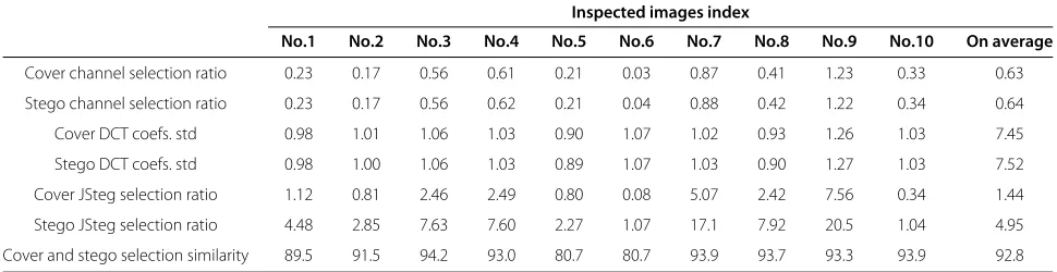
Thus, based on our proposed WF, it is proposed to cat-egorise ‘residual noise’ set into two subsets: ‘non-zero’ subset and ‘zero’ subset. To verify the effectiveness of our improved algorithm, it is proposed to randomly choose ten exemplary images which are compressed to JPEG for-mat images with quality factor 70 and embedding rateR=
0.05. Also, all the images of the BossBase database [27] are used for computing the average value. Table 1 gives the statistical ratio of the data in which the annotations of the table are as follows:
• Cover channel selection ratio: denotes the ratio of the ‘non-zero’ subset to the ‘residual noise’ set of a cover image.
• Stego channel selection ratio: denotes the ratio of the ‘non-zero’ subset to the ‘residual noise’ set of a stego image.
• Cover DCT coefs. std : denotes the standard deviation of the ‘residual noise’ set from a cover image.
• Stego DCT coefs. std : denotes the standard deviation of the ‘residual noise’ set from a stego image.
• Cover JSteg selection ratio: denotes the ratio of the DCT coefficients used by JSteg in the ‘non-zero’ subset to the DCT coefficients used by JSteg in the ‘residual noise’ set from a cover image.
• Stego JSteg selection ratio: denotes the ratio of the DCT coefficients used by JSteg in the ‘non-zero’ subset to the DCT coefficients used by JSteg in the ‘residual noise’ set from a stego image.
• Cover and stego selection similarity: denotes the ratio of the same position in the ‘non-zero’ subset before and after embedding.
Table 1 Ratio (%) comparison before and after embedding
Inspected images index
No.1 No.2 No.3 No.4 No.5 No.6 No.7 No.8 No.9 No.10 On average
Cover channel selection ratio 0.23 0.17 0.56 0.61 0.21 0.03 0.87 0.41 1.23 0.33 0.63
Stego channel selection ratio 0.23 0.17 0.56 0.62 0.21 0.04 0.88 0.42 1.22 0.34 0.64
Cover DCT coefs. std 0.98 1.01 1.06 1.03 0.90 1.07 1.02 0.93 1.26 1.03 7.45
Stego DCT coefs. std 0.98 1.00 1.06 1.03 0.89 1.07 1.03 0.90 1.27 1.03 7.52
Cover JSteg selection ratio 1.12 0.81 2.46 2.49 0.80 0.08 5.07 2.42 7.56 0.34 1.44
Stego JSteg selection ratio 4.48 2.85 7.63 7.60 2.27 1.07 17.1 7.92 20.5 1.04 4.95
Cover and stego selection similarity 89.5 91.5 94.2 93.0 80.7 80.7 93.9 93.7 93.3 93.9 92.8
also show that, after rejection of the content, the ‘resid-ual noise’ standard deviation is very small compared to the original DCT coefficients (see also Figures 2 and 3), which thus permits a better detection of modifications due to JSteg embedding. The ratio of cover and stego selection similarity which is kept at the high value sig-nifies that most of the ‘residual noise’ are chosen at the same position. Then, the only difference is the compar-ison between the cover JSteg selection ratio and stego JSteg selection ratio. It should be noted that if all DCT coefficients used by JSteg are included in the ‘non-zero’ subset, then the ratio equals 100%. It is observed that only a few of the DCT coefficients used by the JSteg algorithm is included in the ‘non-zero’ subset. Neverthe-less, after embedding, the ratio of stego JSteg selection ratiois largely improved, compared with the ratio ofcover JSteg selection ratio. It can be assumed that by using a WF, more ‘residual noise’ from the embedding positions are counted. Besides, prior to embedding secret informa-tion, we never know which position will be embedded; the very low ratio of the cover JSteg selection ratio is reasonable.
By investigating the ‘non-zero’ and ‘zero’ subset, although we can not capture all the embedding positions in the DCT domain, it is totally enough to detect the JSteg steganography. Besides, all the coefficients in the ‘zero’ subset are not counted in our proposed test. On average, for a cover image with the size of 512× 512, 0.63% of the coefficients are kept to compute the test; 0.64% of the coefficients from a stego image are used. As the embed-ding rateR = 0.05, it is obvious that most of the DCT coefficients remain the same before and after embedding. Thus, it is not necessary to compute these values. Fur-thermore, the LR values of these DCT coefficients without embedding any information probably mask or disturb the LR from DCT coefficients with JSteg embedding.
4.4 Design of proposed test
In Section 3, the framework of hypothesis testing theory has been presented assuming that distribution parameters
are known for each DCT coefficient. To design a practical test, a usual solution consists of replacing the unknown parameter by its ML estimation. This leads to the con-struction of a generalised LRT. A similar concon-struction is adopted in this paper, using the ad hoc estimators pre-sented at the beginning of Section 4, instead of using the ML method to estimate the distribution parameters of each DCT coefficient. The proposed test is thus defined as:
δ(U)= ⎧ ⎪ ⎪ ⎪ ⎪ ⎪ ⎨ ⎪ ⎪ ⎪ ⎪ ⎪ ⎩
H0if(U)= K
k=1 64
l=2
cs(uk,l) <τ,
H1if(U)= K
k=1 64
l=2
cs(uk,l)≥τ, (19)
where the channel-selection decision statisticcs(uk,l)=
(uk,l)· wk,l for a single DCT coefficient is given, and a weighting factor wk,l selects the DCT channel. Next, let us study the(uk,l)to verify the effectiveness of our proposed test.
To verify our improvement based on the Laplacian test (see [22]), it is proposed to consider the weighing fac-torwk,l as a constant equal to 1. The scale parameterb is estimated by using MLE and the location parameter is ignored (see details in [22]). The LR is given by:
(uk,l)=log
1+R 2 +
R
2exp
bsign(k)(k− ¯k)
.
(20)
The first improvement of the previous LR is the con-sideration of the location parameterμk,l(see Section 4.1). The new LR is designed by:
1(uk,l)=log
1+R 2+
R
2exp
bsign(k−μk,l)(k− ¯k)
.
The second improvement is the estimation of the scale parameterbk,l (see Section 4.2) and ignore the location parameter. The LR is designed by:
2(uk,l)=log
1+R 2 +
R
2exp
bk,l
sign(k)(k− ¯k)
.
(22)
The third improvement is to give the assumption that DCT coefficients are i. i. d. The scale parameterbk,l and the location parameter μk,l of the distribution are esti-mated separately by using our proposed algorithms in Sections 4.1 and 4.2.
3(uk,l)=log
1+R 2+
R
2exp
bk,l
sign(k−μk,l)(k− ¯k)
.
(23)
Moreover, it is proposed to explore the effectiveness of introducing a weighing factorwk,lwhich is defined as:
wk,l=
0 if k−μk,l∈(−0.5, 0.5)
1 otherwise. (24)
The last LR is obtained by multiplying (23) bywk,l:
cs(uk,l)=3( uk,l)wk,l. (25) It is should be noted that (20) is the algorithm from [22]. In Section 5, the specific comparison of the detectors is presented. In order to have a normalised decision statistic for the whole image,(U)is defined as:
(U)= 1
SL K
k=1 64
l=2
cs(uk,l)−EH0
μk,l,bk,l
withS2L= K
k=1 64
l=2
VH0μk,l,bk,l
.
(26)
4.5 Comparison with prior art
The WS Jpeg, as well as the WS for spatial domain, is based on the underlying assumption that the observations follow a Gaussian distribution. As recently shown [6,8], the WS implicitly assumes that the quantization step is negligible. Let us rewrite the LR test for JSteg detection based on a Gaussian distribution model of DCT coeffi-cients. LetXbe a random variable following a quantized Gaussian distribution. Exploiting the assumption that the quantization step is negligible compared to noise standard deviation allows the writing of:
P[X=k]=
(k+1/2)
(k−1/2)
1
σ√2πexp
−(x−μ)2
2σ2
dx
≈
σ√2πexp
−(k−μ)2
2σ2
. (27)
Putting this expression of the pmf under hypothesis H0 into the LR (2), and assuming that the quantization
step is negligible compared to the noise standard devia-tion, << σ, it is immediate to obtain the following expression of the LR under the assumption of Gaussian distribution of DCT coefficient:
log ⎛ ⎝1+R
2 +
R
2
exp−(k2¯−σ2μ)2
exp−(k2−σ2μ)2
⎞ ⎠
≈ R
2σ2 (k− ¯k) (k−μ) =% &' (wσ % &' (±1 %(k&'−μ)(
(28)
see details in Appendix C. This expression highlights the well-known fact that the WS consists in fact of three terms: 1) the termwσ which is a weight so that pixels or DCT coefficients with the highest variance have a small-est importance, 2) the term(k− ¯k) = ±1 according the LSB ofkand 3) the term(k−μ).
In comparison, the expression of the LR for a Laplacian distribution model (15), as well as the expression of the proposed test with estimates (21) can be approximated by (see details in Appendix B):
R
2b (k− ¯k)sign(k−μ)= %&'(
wb
% &' (
±1 %sign(k&'−μ)( (29)
which is also made of three terms; the two first are roughly similar to the two first terms of the WS : 1) the termwbis a weight so that DCT coefficients with the highest ‘scale’
bhave the smallest importance; note that the variance is proportional tob2; 2) the term(k− ¯k)= ±1 according to the LSB ofk. However, in the expression of the LR based on the Laplacian model, the term(k−μ)of the WS is replaced with its sign. This shows that the statistical tests based on the Laplacian model and based on the Gaussian model are essentially similar.
5 Numerical simulations
5.1 Results on simulated images
One of the main contributions of this paper is to show that the hypothesis testing theory can be applied in practice to design a statistical test with known statistical properties for JSteg steganalysis.
Figure 5Expectationm0and varianceσ02as a function of the
scale parameterbtheoretically and empirically.
moments are almost equal to the analytically established ones.
Subsequently, to verify the effectiveness of the estab-lished LRT δlr(U), again, a Monte Carlo simulation is performed by repeating 10,000 times using a vector 64× 4, 096 following the Laplacian distribution, in which the scale parameter is selected arbitrarily as 3 and the location parameter 0. Under the hypothesisH0 andH1,
respec-tively, Figure 6 presents the comparison between empir-ical and theoretempir-ical distribution of lr(U). The results highlight the validity of the proposed test (10).
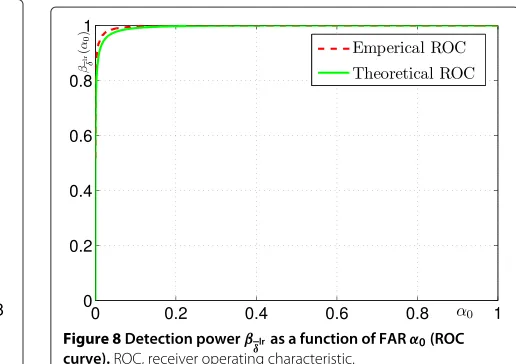
Figure 7 gives the comparison between the empirical and theoretical FARα0, respectively, of the test (10). This particularly demonstrates that two curves are very close. Figure 8 offers the receiver operating characteristic (ROC) comparison, that is the detection powerβδlras a function
of FARα0, of both empirical and theoretical established results in (11) and (12).
Figure 6Comparison between empirical and theoretical
distribution oflr(U).
Figure 7FARα0as a function of the thresholdτlr.
5.2 Results on real images
Another contribution of this paper is to design the optimal test with estimated parameters to break JSteg algorithm in a practical case.
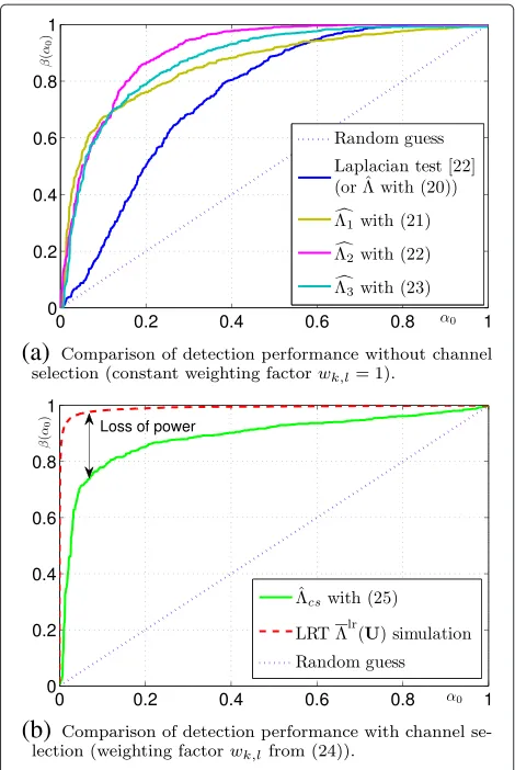
First, let us investigate our proposed detectors (21) to (23). It is proposed to perform a numerical simulation over the 1,000 images from BossBase [27] which have been compressed in JPEG with quality factor 70. The payload, or embedding rate,Ris set at 0.05 for JSteg algo-rithm. For a fair comparison with the detector from [22], it first shows the improvement provided by the proposed model withwk,l = 1. As Figure 9a illustrates, all the pro-posed detectors outperform(u k,l)(20) proposed by [22]. Moreover, in the following investigation, it is proposed to use cs(uk,l) (25). Then, it is proposed to give the per-formance of this detector on 1,000 simulated images in which a DCT subband is generated by strictly following the Laplacian distribution (see Figure 9b). Then, a com-parison with simulations of the LR test shows the loss of power due to the estimation of expectation and scale
Figure 8Detection powerβ
(a)
(b)
Figure 9ROC curves comparison, detection power as a function of FARα0.(a)Comparison of detection performance without
channel selection (constant weighting factorwk,l=1).(b)
Comparison of detection performance with channel selection (weighting factorwk,lfrom (24)). LRT, likelihood ratio test.
parameters. It should be noted that in all our proposed detectors in this paper, ( uk,l) (23) with wk,l (24) per-forms best. Thus, it is proposed to use it as our optimal steganalyser for competing with the state-of-the-art JSteg detectors. It is should be emphasised that in Figure 9, the wavelet denoising filter [43] is used for estimating the location parameterμk,l(see Section 4.1).
To verify the relevance of the proposed methodology, it is proposed to compare the proposed statistical test with two other detectors. The first chosen competitor is the statistical test proposed in [22] as it is also based on a Laplacian model but does not take into account the dis-tribution parameters as nuisance parameters; it considers that DCT coefficients are i. i. d. , following a Laplacian distribution with zero mean. The comparison with this test is meaningful as it allows us to measure how much the detection performance is improved by removing the assumption that the DCT coefficients of each subband are
i. i. d. The second chosen competitor is the WS [15] due to its similarity with the proposed statistical test, see details in Section 4.5.
For a large-scale verification, it is proposed to use the ‘break our steganographic system’ (BOSS) database, made of 10,000 grayscale images of size 512×512 pixels, used with payload R = 0.05. Prior to our experiments, the images have been compressed in JPEG using the linux command convert which uses the standard quantization table. Note also that all the JSteg steganography was per-formed using a Matlab source code we developed based on Phil Sallee’s Jpeg Toolboxf. Four denoising methods have been tested to estimate the expectation of each DCT coefficient, namely the K-SVD, the BM3D, the NL means and the wavelet denoising algorithms.
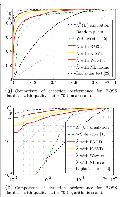
Figure 10 shows the detection performances obtained over the BOSS database compressed with quality fac-tor 70. The detection performances are shown as ROC curves, that is the detection power is plotted as a function of false alarm probability. Figure 10a particularly empha-sises that the statistical test based on the Laplacian model does not perform well while the proposed methodology which takes into account that the Laplacian distribution parameters as nuisance parameters allows us to largely improve the performance. Similarly, the WS detector achieves overall good detection performance. However, it can be shown in Figure 10b, which presents the same results using a logarithmic scale, that for low false alarm probabilities, the performance of the WS significantly decreases. On the opposite, the proposed statistical test still performs well.
Among the four denoising algorithms that have been tested, the BM3D achieves the best performance, but it can be observed in Figure 10 that the performances obtained using the K-SVD and using the wavelet denois-ing methods are also very good. The performance of NL means method is comparable with the WS detector [15].
To extend the results previously presented, a similar test has been performed over the BOSS database using the quality factor 85. The detection performance obtained by the proposed test and by the competitors are pre-sented in Figure 11. Again, this figure shows that based on the Laplacian model, the statistical test assuming that DCT coefficients of a subband are i. i. d. has an unsat-isfactory performance. It can also be noted that even though the WS performs slightly better for low false alarm probability, compared to the results obtained with qual-ity factor 70, it performs much worse than the proposed statistical test.
6 Conclusions
(a)
(b)
Figure 10Comparison of detection performance for BOSS database with quality factor 70.(a)Comparison of detection performance for BOSS database with quality factor 70 (linear scale). (b)Comparison of detection performance for BOSS database with quality factor 70 (logarithmic scale). WS, weighted stego-image. It is noted that denoising filters are respectively designed based on wavelet, block-matching and 3D (BM3D), dictionary learning (K-SVD) and non-local (NL) means algorithms.
is used as a statistical model of DCT coefficients, but opposed to what is usually proposed, it is not assumed that all DCT coefficients from a subband are i. i. d. This leads us to consider the Laplacian distribution parame-ters, namely the expectationeand the scale parameterb, as nuisance parameters as they have no interest for the detection of hidden data, but they must be carefully taken into account to design an efficient statistical test. Numeri-cal results show that by estimating those nuisance param-eters, the Laplacian model allows the designing of an accurate statistical test which outperforms the WS detec-tor. The comparison with the optimal detector based on the Laplacian model and on the assumption that all DCT
Figure 11Comparison of detection performance for BOSS database with quality factor 85 (logarithmic scale).It is noted that denoising filters are respectively designed based on wavelet, block-matching and 3D (BM3D), dictionary learning (K-SVD) and non-local (NL) means algorithms.
coefficients of a subband are i. i. d. shows the relevance of the proposed approach.
A possible future work would be to apply this approach with a state-of-the-art statistical model of DCT coeffi-cients, such as the generalized Gaussian or the gener-alized gamma model. This could provide improvements in the detection performance at the cost of a higher complexity.
Endnotes
aIn this paper, we assume, without loss of generality,
that both width and height of the inspected image are multiples of 8.
bIn practice, DCT coefficients belong to set
[−1024,. . ., 1023], see [22].
cNote that we refer to the Lindeberg’s CLT, whose
conditions are easily verified in our case, because the random variable are independent but are not i. i. d. .
dImage Processing On-Line journal is available at:
http://www.ipol.im
eSource codes are available at: http://dde.binghamton.
edu
fPhil Sallee’s Jpeg Toolbox is available at: http://dde.
binghamton.edu/download/jpeg_toolbox.zip
Appendix
A Quantized Laplacian pmf
LetXbe a Laplacian random variable with expectationμ and varianceb. Its pdf is thus (see (13)):
fμ,b(x)= 1 2bexp
−|x−μ| b
and a straightforward calculation shows that its cdf is given by:
Fμ,b(x)= 1 2 +
1
2sign(x−μ)
1−exp
−|x−μ| b , (30) = 1 2exp x−μ
b
if x< μ,
1− 12exp−x−bμ if x≥μ. (31)
Now consider the result from quantization of this ran-dom variableY = X/, it is immediate to establish the pmf of this random variable. Let us first consider the case
(k+1/2) < μ(due to the symmetry of Laplacian pdf, the case(k−1/2) > μis treated similarly).
The pmf ofYis given by:
P[Y=k]=P[(k−1/2)≤X< (k+1/2)] ,
= 1
2exp
(
k+1/2)−μ b
− 1
2exp
(k−1/2)−μ
b a
,
= 1
2exp
k−μ
b exp 2b − 1 2exp
k−μ b exp − 2b , =exp
k−μ
b sinh 2b ,
Applying similar calculations for case(k−1/2) > μ, one gets:
P[Y =k]=exp
−|k−μ|
b sinh 2b , (32)
which corresponds to the pmf given in Equation (14). The case(k−1/2) < μ < (k+1/2)is treated similarly.
C Log-likelihood ratio calculation
By putting the expression of quantized Laplacian pmf (32) into the expression of the LR (7), it is immediate to write:
lr(u
k,l)=log ⎛ ⎝1−R
2+
R
2
exp−|k¯b−μ|sinh2b exp
−|k−μ|
b
sinh2b ⎞ ⎠.
Let us study the term:
exp−|k¯b−μ|sinh2b
exp−|kb−μ|sinh2b=
exp−|k¯b−μ|
exp−|kb−μ| ,
=exp
−|k+(k¯−k)−μ| b
exp−|kb−μ| ,
=exp
−|k−μ| b
expsign(kb−μ)(k−¯k)
exp−|kb−μ|
,
=exp
sign(k−μ)(k− ¯k) b
.
(33)
From this Equation (33), it is immediate to establish the expression (15):
log
1− R 2 +
R
2exp
sign(k−μ)(k− ¯k) b
.
By using a Taylor expansion, lr(uk,l) can be approxi-mated by:
log
1−R 2+
R
2
1+sign(k−μ)(k− ¯k)
b ≈log 1+
Rsign(k−μ)(k− ¯k)
2b
,
≈ R
2b(k− ¯k)sign(k−μ).
B LR based on the Gaussian model (WS)
LetXbe a Gaussian random variable with expectationμ and varianceσ2. Define the quantized Gaussian random variable as follows:Y= X/; its pmf is given byPμ,σ = {pμ,σ[k]}∞k=−∞with:
pμ,σ[k]=P[Y=k] = (k+1/2)
(k−1/2)
1
σ√2πexp
−(x−μ)2
2σ2
dx.
Assuming that the quantization stepis ‘small enough’ compared to the variance << σ, it holds true that [6,44]:
pμ,σ[k]≈
σ√2πexp
−(k−μ)2
2σ2
, (34)
and
pμ,σ[k]+pμ,σ[k¯]≈ 2
σ√2πexp ⎛ ⎜ ⎜ ⎜ ⎜ ⎜ ⎝ −
k+¯k
2 −μ
2
Let us rewrite the LR for the detection of JSteg (7) as follows
lr(u
k,l)=log
1−R 2 +
R
2
pμ,σ[k¯] pμ,σ[k]
,
=log
1−R+ R
2
pμ,σ[k¯]+pμ,σ[k] pμ,σ[k]
. (36)
Using the expressions (34) and (35) let us study the follow-ing ratio:
pμ,σ[k]¯ +pμ,σ[k] pμ,σ[k] =2
exp
−(
k+¯k)
2 −μ 2
2σ2
exp−(k2−σ2μ)2
, =2 exp −
k−μ+/2(k¯−k)2
2σ2
exp
−(k−μ)2 2σ2
,
=2 exp
−(k−μ)2 2σ2
exp
(k−μ)(k−¯k)
2σ2
exp
−2 8σ2
exp
−(k−μ)2 2σ2
,
=2 exp
(k−μ)(k− ¯k) 2σ2
exp
−2 8σ2
.
(37)
Putting the expression (37) into the expression of the log-LR (36) immediately gives:
lr(u
k,l)=log
1+R
exp
(k−μ)(k− ¯k)
2σ2
×exp
−2
8σ2
−1
(38)
from which is a Taylor expansion around/σ = 0, this results from the assumption that << σ, and finally gives the well-known expression of the WS:
lr(u
k,l)≈R 2σ2
k− ¯kx(k−μ) (39)
Competing interests
The authors declare that they have no competing interests.
Authors’ contributions
TQ carried out the main research of this work and drafted the manuscript. FR, RC and CZ helped to modify the manuscript. All authors read and approved the final manuscript.
Acknowledgements
The Matlab codes will be published upon paper acceptance. The work of FR, RC and CZ is funded by Troyes University of Technology (UTT) strategic program COLUMBO. The PhD thesis of TQ is funded by the China Scholarship Council (CSC) program.
Received: 10 November 2014 Accepted: 10 February 2015
References
1. R Böhme,Advanced Statistical Steganalysis. (Springer, New York, 2010) 2. J Fridrich,Steganography in Digital Media: Principles, Algorithms, and
Applications. (Cambridge University Press, Cambridge, 2009) 3. I Cox, M Miller, J Bloom, J Fridrich, T Kalker,Digital Watermarking and
Steganography. (Morgan Kaufmann, Burlington, 2007)
4. J Fridrich, J Kodovsk`y, inInformation Hiding. Steganalysis of LSB replacement using parity-aware features (Springer, New York 2013), pp. 31–45
5. T Zhang, X Ping, inProceedings of the 2003 ACM Symposium on Applied Computing. A fast and effective steganalytic technique against jsteg-like algorithms (ACM, New York 2003), pp. 307–311
6. R Cogranne, C Zitzmann, L Fillatre, F Retraint, I Nikiforov, P Cornu, in
Information Theory Proceedings (ISIT), 2011 IEEE International Symposium On. Statistical decision by using quantized observations (IEEE, New York 2011), pp. 1210–1214
7. R Cogranne, C Zitzmann, L Fillatre, F Retraint, I Nikiforov, P Cornu, in
Information Hiding. A cover image model for reliable steganalysis (Springer, New York 2011), pp. 178–192
8. C Zitzmann, R Cogranne, F Retraint, I Nikiforov, L Fillatre, P Cornu, in
Information Hiding. Statistical decision methods in hidden information detection (Springer, New York 2011), pp. 163–177
9. J Fridrich, M Goljan, R Du, inProceedings of the 2001 Workshop on Multimedia and Security: New Challenges. Reliable detection of LSB steganography in color and grayscale images (ACM, New York 2001), pp. 27–30
10. S Dumitrescu, X Wu, Z Wang, Detection of LSB steganography via sample pair analysis. Signal Process. IEEE Trans.51(7), 1995–2007 (2003) 11. AD Ker, P Bas, RBöhme, R Cogranne, S Craver, T Filler, J Fridrich, T Pevn`y, in
Proceedings of the First ACM Workshop on Information Hiding and Multimedia Security. Moving steganography and steganalysis from the laboratory into the real world (ACM, New York 2013), pp. 45–58 12. J Fridrich, M Goljan, inElectronic Imaging 2004. On estimation of secret
message length in LSB steganography in spatial domain (International Society for Optics and Photonics Washington, 2004), pp. 23–34 13. O Dabeer, K Sullivan, U Madhow, S Chandrasekaran, B Manjunath,
Detection of hiding in the least significant bit. Signal Process. IEEE Trans.
52(10), 3046–3058 (2004)
14. AD Ker, R Böhme, inElectronic Imaging 2008. Revisiting weighted stego-image steganalysis (International Society for Optics and Photonics Washington, 2008), pp. 681905–681905
15. R Böhme, inInformation Hiding. Weighted stego-image steganalysis for JPEG covers (Springer, New York 2008), pp. 178–194
16. R Cogranne, C Zitzmann, F Retraint, IV Nikiforov, P Cornu, L Fillatre, A local adaptive model of natural images for almost optimal detection of hidden data. Signal Process.100, 169–185 (2014)
17. EY Lam, JW Goodman, A mathematical analysis of the DCT coefficient distributions for images. Image Process. IEEE Trans.9(10), 1661–1666 (2000)
18. F Muller, Distribution shape of two-dimensional DCT coefficients of natural images. Electron. Lett.29(22), 1935–1936 (1993)
19. J-H Chang, JW Shin, NS Kim, SK Mitra, Image probability distribution based on generalized gamma function. Signal Process. Lett. IEEE.
12(4), 325–328 (2005)
20. P Sallee, Model-based methods for steganography and steganalysis. Int. J. Image Graph.5(01), 167–189 (2005)
21. R Böhme, A Westfeld, Breaking cauchy model-based JPEG steganography with first order statistics. Computer Security–ESORICS, 125–140 (2004) 22. C Zitzmann, R Cogranne, L Fillatre, I Nikiforov, F Retraint, P Cornu, in
Acoustics, Speech and Signal Processing (ICASSP), 2012 IEEE International
Conference On. Hidden information detection based on quantized
Laplacian distribution (IEEE, New York 2012), pp. 1793–1796
23. J Kodovsky, J Fridrich, Quantitative structural steganalysis of jsteg. Inform. Forensics Secur. IEEE Trans.5(4), 681–693 (2010)
24. K Lee, A Westfeld, S Lee, inDigital Watermarking. Category attack for LSB steganalysis of JPEG images (Springer, New York 2006), pp. 35–48 25. S Lyu, H Farid, Steganalysis using higher-order image statistics. Inform.
26. T Pevny, J Fridrich, Multiclass detector of current steganographic methods for JPEG format. Inform. Forensics Secur. IEEE Trans.3(4), 635–650 (2008) 27. P Bas, T Filler, T Pevný, inInformation Hiding, 13th International Workshop, ed. by Filler T. Break our steganographic system — the ins and outs of organizing boss (IEEE, New York 2011)
28. T Denemark, V Sedighi, V Holub, R Cogranne, J Fridrich, inIEEE Workshop on Information Forensic and Security, Atlanta, GA. Selection-channel-aware rich model for steganalysis of digital images (IEEE, New York 2014) 29. W Tang, H Li, W Luo, J Huang, inProceedings of the 2nd ACM Workshop on
Information Hiding and Multimedia Security. Adaptive steganalysis against WOW embedding algorithm (ACM, New York 2014), pp. 91–96 30. T Qiao, C Ziitmann, R Cogranne, F Retraint, inProceedings of the 2nd ACM
Workshop on Information Hiding and Multimedia Security. Detection of jsteg algorithm using hypothesis testing theory and a statistical model with nuisance parameters (ACM, New York 2014), pp. 3–13
31. T Qiao, C Zitzmann, R Cogranne, F Retraint, inIEEE International Conference on Image Processing (ICIP). Statistical detection of jsteg steganography using hypothesis testing theory (IEEE New York, 2014), pp. 5517–5521 32. J Nakamura,Image Sensors and Signal Processing for Digital Still Cameras.
(CRC Press, Boca Raton, 2005)
33. WB Pennebaker, JL Mitchell,JPEG: Still Image Data Compression Standard. (Springer, Germany, 1993)
34. D Upham, Jsteg steganographic algorithm 1999 Available on the internet. http://www.filewatcher.com/m/jpeg-jsteg-v4.diff.gz.8878-0.html 35. EL Lehmann, JP Romano,Testing Statistical Hypotheses. (Springer,
Germany, 2006)
36. TH Thai, R Cogranne, F Retraint, inICIP. Steganalysis of Jsteg algorithm based on a novel statistical model of quantized DCT coefficients (IEEE, New York 2013), pp. 4427–4431
37. T Thai, R Cogranne, F Retraint, Statistical model of quantized DCT coefficients: Application in the steganalysis of jsteg algorithm. IEEE Trans. Image Process. Publ. IEEE Signal Process. Soc.23(5), 1980-1993 (2014) 38. R Cogranne, F Retraint, An asymptotically uniformly most powerful test
for LSB matching detection. IEEE Trans. Information Forensics and Security. Publ. IEEE Signal Process. Soc.8(3), 464-476 (2013)
39. TH Thai, F Retraint, R Cogranne, inImage Processing (ICIP) 2012 19th IEEE International Conference On. Statistical model of natural images (IEEE New York, 2012), pp. 2525–2528
40. M Lebrun, An analysis and implementation of the BM3D image denoising method. Image Processing On Line.2, 175-213 (2012)
41. M Lebrun, A Leclaire, An implementation and detailed analysis of the K-SVD image denoising algorithm. Image Processing On Line.2, 96-133 (2012)
42. A Buades, B Coll, J-M Morel, inComputer Vision and Pattern Recognition, 2005. CVPR 2005. IEEE Computer Society Conference On. A non-local algorithm for image denoising, vol. 2 (IEEE New York, 2005), pp. 60–65 43. J Lukas, J Fridrich, M Goljan, Digital camera identification from sensor
pattern noise. Inform. Forensics Secur. IEEE Trans.1(2), 205–214 (2006) 44. R Cogranne, F Retraint, C Zitzmann, I Nikiforov, L Fillatre, P Cornu, Hidden
information detection using decision theory and quantized samples: Methodology, difficulties and results. Digital Signal Process.24, 144–161 (2014)
Submit your manuscript to a
journal and benefi t from:
7Convenient online submission
7Rigorous peer review
7Immediate publication on acceptance
7Open access: articles freely available online
7High visibility within the fi eld
7Retaining the copyright to your article