DOI10.1186/2190-8567-3-7
R E S E A R C H Open Access
Transient Localized Wave Patterns and Their
Application to Migraine
Markus A. Dahlem·Thomas M. Isele
Received: 9 November 2012 / Accepted: 15 May 2013 / Published online: 29 May 2013
© 2013 M.A. Dahlem, T.M. Isele; licensee Springer. This is an Open Access article distributed under the terms of the Creative Commons Attribution License (http://creativecommons.org/licenses/by/2.0), which permits unrestricted use, distribution, and reproduction in any medium, provided the original work is properly cited.
Abstract Transient dynamics is pervasive in the human brain and poses challeng-ing problems both in mathematical tractability and clinical observability. We investi-gate statistical properties of transient cortical wave patterns with characteristic forms (shape, size, duration) in a canonical reaction-diffusion model with mean field inhi-bition. The patterns are formed by ghost behavior near a saddle-node bifurcation in which a stable traveling wave (node) collides with its critical nucleation mass (sad-dle). Similar patterns have been observed with fMRI in migraine. Our results support the controversial idea that waves of cortical spreading depression (SD) have a causal relationship with the headache phase in migraine and, therefore, occur not only in migraine with aura (MA), but also in migraine without aura (MO), i.e., in the two major migraine subtypes. We suggest a congruence between the prevalence of MO and MA with the statistical properties of the traveling waves’ forms according to which two predictions follow: (i) the activation of nociceptive mechanisms relevant for headache is dependent upon a sufficiently large instantaneous affected cortical area; and (ii) the incidence of MA is reflected in the distance to the saddle-node bi-furcation. We also observed that the maximal instantaneous affected cortical area is anticorrelated to both SD duration and total affected cortical area, which can explain why the headache is less severe in MA than in MO. Furthermore, the contested notion of MO attacks with silent aura is resolved. We briefly discuss model-based control and means by which neuromodulation techniques may affect pathways of pain for-mation.
Electronic supplementary materialThe online version of this article (doi:10.1186/2190-8567-3-7) contains supplementary material.
M.A. Dahlem (
)Department of Physics, Humboldt-Universität zu Berlin, Berlin, Germany e-mail:[email protected]
T.M. Isele
1 Introduction
The undoubtedly most fundamental example of transient dynamics is the phe-nomenon of excitability, that is, all-or-none behavior. Shortly after transient response properties of excitable membranes were classified into two classes [1], it was also explained in a detailed mathematical model how excitability emerges from electro-physiological properties of such membranes in the ground-breaking work by Hodgkin and Huxley [2]. Two features are central and are by no means exclusive to biologi-cal membranes but shared by all excitable elements. Firstly, the inevitable threshold in any all-or-none behavior requires nonlinear dynamics. Secondly, the transient re-sponse of the system to a super-threshold stimulation eventually has to lead back to a globally stable steady state after some large phase space excursion. This indicates global dynamics, that is, dynamics involving not only fixed points and their local bi-furcations but more complex invariant sets, for instance periodic orbits that collide with fixed points. An excitable element is in some sense the washed-up brother of the relaxation oscillator: When the threshold vanishes, a single excitable element usu-ally becomes a simpler behaved—and much longer known—relaxation oscillator [3]. Vice versa, when a saddle-node disrupts a limit cycle and introduces a threshold, the sustained oscillations are reduced to long transient responses after perturbations, that is, the dynamics becomes excitable. In this study, we utilize a similar scenario to dis-rupt sustained traveling wave solutions in a spatially extended medium such that only transient waves occur. We investigated statistical properties of these transient waves to gain a dynamical understanding of spontaneous episodes in migraine.
We will briefly introduce concepts of excitable elements and excitable media in two-variable reaction-diffusion systems. While we also introduce migraine, the view of migraine as a dynamical disease is more elaborated in the discussion in Sect.5. A particular focus is set on the idea to introduce an global inhibitory feedback that is also studied in various other systems outside the neurosciences and also in neural field models. Section2sets the stage for our canonical model introduced in Sect.3 from were we proceed to our results on the statistical properties of transient waves in Sect.4.
2 Motivation of a Macroscopic Model for Migraine Aura
2.1 Spatiotemporal Behavior of Excitable Systems
Excitability was first described for neurons in the original conductance-based membrane model by Hodgkin and Huxley [2]. This and many more refined versions of neural excitability to date contain four or more dynamic variables, but fortunately this is not essential for excitable systems. In fact, it turned out for excitable elements that the main two classes of excitability are actually amenable to direct analysis in a two-dimensional phase plane by identifying in the conductance-based model fast and slow processes and grouping these into dynamics of just two lump variables [4, 5]. Using such a geometrical approach and partly analytical theory, the original em-pirical classification of excitability was further pursued with bifurcation analysis [6], explaining class I by identifying its threshold as a stable manifold of a saddle point on an invariant cycle and the threshold of class II as a trajectory from which nearby trajectories diverge sharply (called canard trajectory). Extensions to these principal mechanisms involve codimension 2 bifurcations and lead also to bursting in three-variable models, which have been investigated in great detail [7]. However, the two-variable models of a fast activator and slow inhibitor and their phase portraits of class I and II became qualitative prototypes for excitable elements in various biological [8], chemical [9], and physical contexts [10].
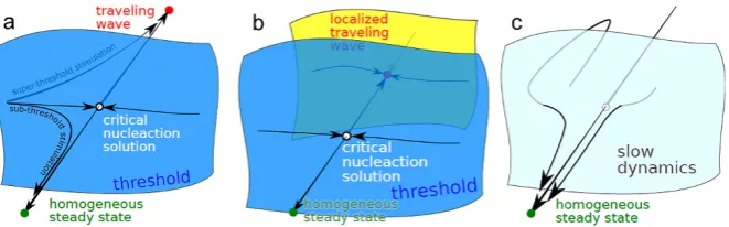
Distinct from excitable elements and their classification are spatially extended ex-citable media. Already the original work by Hodgkin and Huxley [2] described spa-tially extended, tube-like membranes (axons) and introduced the cable equation as a parabolic partial differential equation, which is in the same class as the diffusion equation. In this reaction-diffusion framework, an excitable medium is the continuum limit of a locally coupled chain of excitable elements. Even in reaction-diffusion media with infinite-dimensional phase space, we can again apply geometrical ap-proaches, simply because excitable media are not defined by—in contrast to excitable elements—transient dynamics but traveling wave solutions. The quiescent state is the nonexcited homogeneous steady state. And like the quiescent state, excited states of a medium are usually stationary states in some appropriate comoving frame, for ex-ample, along thex-direction withξ =x−ct. Furthermore, the threshold is related to an unstable stationary state, the critical nucleation solution, usually in another co-moving frame includingc=0. The existence of the nucleation solution is a simple consequence of multistability; see Fig.1a, but note that even monostable excitable elements have similar unstable stationary states in class I.
In this study, we propose a spatially extended model for wave-like patterns with a characteristic shape, size, and duration. These patterns are (spatially confined) tran-sient responses to confined, spatially structured perturbations of the globally sta-ble homogeneous steady state. These transient responses—after propagating for a while—will always eventually approach the homogeneous state. This leads to a new type of local excitability in a spatially extended medium involving transient travel-ing wave solutions as invariant sets. Both the model and the initial conditions are motivated by the pathophysiology of migraine and clinical observations [11–13].
2.2 Cortical Activity Pattern and Neurovascular Coupling During Migraine
associ-Fig. 1 Schematic sketch of the orbit structure in phase space.aExcitable media with activator–inhibitor kinetics; the activator diffuses and the inhibitor is immobilized. These systems are multistable, the quies-cent state is the homogeneous steady state (green dot), and at least one traveling wave solution must exit as the excited state (red dot). The basins of attraction between these states are separated by the stable man-ifold (blue) of a critical nucleation solution (white dot). Such solutions have only one unstable direction; the corresponding unstable manifold consists of two heteroclinic connections to the stable solutions (green and red dots).bExcitable media with one activator and two inhibitors, one of which is immobilized, the other fast diffusing or realized by mean field inhibition. The orbit structure in phase space is similar to abut the traveling wave solution is now localized similar to the critical nucleation solution to which it is connected.cMedium that lost spatial excitability, that is, traveling wave solutions do not exist. Note that the traveling wave solution disappears by a collision of the traveling wave solution with its nucleation solution, that is, in a saddle-node bifurcation. Such systems show ghost behavior, which influences the dynamics in form oflocalexcitability (see text)
ated with nausea, vomiting, and sensitivity to light, sound, and even movement [14]. Migraine with aura (MA) involve in addition, but also rarely exclusively, neurologic symptoms (aura) that are caused by waves of cortical spreading depression [12,15– 17].
Spreading depression (SD) is a massive but temporary perturbation of ion home-ostasis due to seizure-like discharges of neurons. The ion concentrations are usu-ally kept with a narrow range of acceptable limits, while during SD ion concentra-tions can change by over one order of magnitude to a nearly complete depletion of transmembrane chemical gradients. The ignition of this perturbed ionic balance can spread by diffusion of ions in the extracellular space. Essentially, SD is a slow (about 3 mm/min=50μm/sec) reaction-diffusion wave in the approximate 2D cortical sheet of gray matter.
The cortical tissue SD traverses is functionally impaired causing the neurological migraine aura symptoms, like visual hallucinations [11]. Whether SD is also a key to the subsequent headache phase is an open question, in particular, in cases of migraine without aura (MO). If SD occurs in MO, the massive ionic imbalance must remain clinically silent [18,19] or—by definition of diagnostic criteria—neurological symp-toms must last less than 5 min.
the still contested notion of “silent aura” [22]: Blood-flow changes where observed that were most likely the result of SD.
SD in the cortex is accompanied by a pronounced increased regional cerebral blood flow for about 2 min and a long lasting (∼2 h) decrease [23]. This naturally raises the question of the physiological relevance of these blood-flow changes. Are they just an epiphenomenon that can be used to indirectly measure SD or do these changes participate in the pattern forming mechanism of SD? We suggest that the initial increase in cerebral blood flow for about 2 min is effectively an inhibitory feedback mechanism for SD. The hyperemic phase (increased blood flow) engulfs large regions of the human cortex [16], while, as we further investigate in this study, the massive ionic imbalance directly due to SD is much more limited in extent [12, 13]. This suggests that the inhibitory feedback by neurovascular coupling is a global control mechanism of the neural reaction-diffusion system.
The pattern forming interactions are described in the next section from a mathe-matical perspective. We end this section by providing some background of the phys-iological bases of the spatial mismatch between the more globally increased blood flow (hypermia) and more spatially confined ionic imbalance during SD.
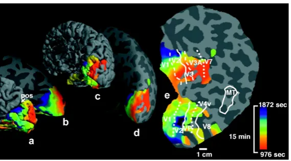
The neural activity and subsequent changes in blood flow are closely coupled called neurovascular coupling. Not only the magnitude but also the spatial loca-tion of blood flow changes reflect neural activity, a fact that is used in noninvasive brain imaging techniques such as functional magnetic resonance imaging (fMRI). SD, however, is a pathological state in which this coupling is to some degree im-paired, in particular evoking long lasting decreases phase (oligemia). To measure the spatial confinement of SD in human cortex during a migraine attack with fMRI, not merely hypermia, but also several other characteristic neurovascular events were used that resemble SD, among others [12]: the initial hyperemia with a character-istic duration followed by oligemia with recovery to baseline, the charactercharacter-istic ve-locity of these events, and a concurrent recovery of stimulus driven activation (see Fig.2).
While the pathological activity of neurons during SD is mainly characterized by a depressed state with literally no activity—hence the name, in the tissue ahead of SD, high-frequency activity and increased synaptic noise has been recorded [24]. The tis-sue surrounding the current location of SD is functionally connected through lateral neural networks with neurons that undergo seizure-like discharging at the rising front of SD. This provides an electrical signal transmission pathway several orders faster than SD, that is, in a first approximation an instantaneous connection. As firstly sug-gested by Wilkinson [25], the feed-forward and feedback cortical circuitry can also explain a more global hypermia by neural and synaptic activation in adjacent cortical areas, which might be mistaken as the area SD traverses, when only hypermia is used to estimate the spatial extend of SD in human cortex during a migraine attack with noninvasive imaging.
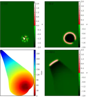
Fig. 2 Source localization of the magnetic resonance (MR) data signal of SD (from [12]). Color code: time from onset, locations showing the first MR signals of SD are coded inred, later times are coded by
green and blue(seecolor scale to the right). Signals from the first 975 seconds were not recorded because the migraine attack was triggered outside the MR imaging facility.aThe data on folded right posterior pole hemispheric cortex;bthe same data on inflated cortical surface;canddthe same data shown on the entire hemisphere from posterior-medial view (oblique forward facing), folded and inflated, respectively. As described in the original study [12], MR data were not acquired from the extreme posterior tip of the occipital pole (rearmost portion).eA fully flattened view of the cortical surface. The aura-related changes are localized wave segments. Note that in the flattened cortex was cut along the steep sulcus calcarine to avoid large area distortions induced by the flattening process. Thecolored border to the leftis the cut edge that should be considered being connected such that the color match up as seen inbandd. Copyright (2001) National Academy of Sciences, USA [12]
mean field feedback. It is reasonable to assume that the larger SD spreads out, the large the increase in neural activity in the surrounding tissue and subsequent hyper-mia with neuroprotective effect. The coupling between increased neural activity and subsequent changes in cerebral blood flow has a significant time delay in the order of seconds, which we ignore for the sake of simplicity in our model.
3 Design of a Macroscopic Model for Migraine Aura
3.1 Model Equations
The canonical model for excitable media are the well-known FitzHugh–Nagumo equations [26] with diffusion in the activator variable:
ε∂u ∂t =u−
1 3u
3−v+ ∇2u,
∂v
∂t =u+β.
(1)
The parameterεseparates the timescales of the dynamics of the activatoruand the inhibitorv, andεis taken to be small. In the present work, we use a value ofε=0.04. The parameterβ is a threshold value which determines from which activator level on the inhibitor concentration is rising. The local dynamics of Eq. (1) (i.e., without the diffusion term) is oscillatory for|β|<1 and excitable for|β|>1. At|β| =1, the local dynamics undergo a supercritical Hopf-bifurcation. We choose a value of
β=1.1 throughout this work. To integrate Eq. (1), we used a simulation based on spectral methods [27] and adaptive timestepping.
We define the (instantaneous) wave size as the area with activator leveluover a certain thresholdu0:
S(t ):= Hu(x, y, t )−u0
dxdy, (2)
whereH is the Heaviside function and we choseu0=0.
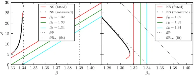
Equations (1) are a paradigmatic model of an excitable medium even beyond neu-roscience [28]. They possess a stable homogeneous solution as well as stable excited states (pulses, spirals, or double spirals) cf. [29,30]. The boundary separating the basins of attraction of these types of solution is given by the stable manifold of the so-called “nucleation-solutions” (NS) whose stability is of saddle-type with one un-stable direction; see Fig.1. These nucleation-solutions are localized areas of excita-tion, which are traveling at uniform speed without changing shape. The size of these solutions, in the sense of Eq. (2), depends on the parametersβ andε. In Fig.3, the sizeSof these nucleation solutions is plotted againstβ. This solution branch is also called∂R and the parameter value for which it diverges is called∂R∞or the “ro-tor boundary” (see next section). Of course, one could also use a measure different fromSfor visualizing the branch∂R, e.g., the propagation speed of the nucleation solution.
To obtain solutions lying on∂R, we used a pseudo-continuation procedure, which is described below.
Making the parameterβ dependent on the wave sizeSadds a mean field control to the system.
β=β(t )=β0+K·S(t ), (3) whereKandβ0are control parameters.
Fig. 3 Left: TheS−β plane with nucleation solution NS, propagation boundary∂P, rotor boundary ∂R∞, and control lines for the used values ofβ0.Right: TheS−β0plane with the same quantities
S is stabilized, cf. [31]. This is visualized in a movie; see Supplementary Material Video 1. This can be understood intuitively, as the stable manifold of a point on∂R
separates the attraction basin of the homogeneous solution for whichSshrinks until
S=0 and the attraction basin of rotating spirals with growingS→ ∞. Imagine the system to be on∂R, that is, showing a nucleation solution as discussed above. If the current state is perturbed to have slightly smallerS, in the uncontrolled system we would have entered the attraction basin of the homogeneous solution (cf. Fig.3). The control however forces the system to stay on the line defined by Eq. (3). If this line intersects∂R, a slightly smallerSmakes the control adjust the value ofβto smaller values, taking the system into the attraction basin of the spiral waves, whereS will grow. The same process happens with different signs if the current state is perturbed to have slightly smallerSthus in effect stabilizing the (one unstable direction of) the nucleation solution.
The aim of the present work is to shed light on the transient behavior, occurring when the control line, Eq. (3) is close to ∂R but does not intersect it as the ones depicted in Fig.3.
To account for the imprecision in∂Rof the simulation and the exact∂R, we mea-sured the∂R in our simulation using a pseudo-continuation procedure. For this, we set the control such that it intersects∂R, and thus stabilize an otherwise unstable solu-tion on it. Letting the simulasolu-tion run until the system has stopped fluctuating, saving the(β, S)-pair, changing the control slightly and doing things over yields points of
∂R in our system. From this measured ∂R and the propagation boundary∂P, in-ferred from continuation in 1D, we chose 3 suitable control lines which were used for simulations in this work:
K=0.003,
β0∈ {1.32,1.33,1.34}.
(4)
branch of nucleation solutions (inβ−S space) to a function of the form β=a+
b
cS+S2 (wherea, b, andcare the fit parameters). We have not only used this function
for visualizing the saddle-node bifurcation, but we also deduced an approximateβ
value for the rotor boundary∂R∞by lettingS→ ∞.
3.2 Effect of Mean Field Inhibitory Feedback Control
The diversity of the behavior of traveling waves in two spatial dimensions was stud-ied in canonical models depending on the two generic parametersβ andεin Eq. (1), which determine the parameter plane of excitability without mean field inhibitory feedback [32]. In those media, patterns of discontinuous (open ends) and spiral-shaped waves are used to probe excitability. These spiral patterns are closely related to the discontinuous, localized transient waves we propose in our model. In fact, the effect of mean field inhibitory feedback control can best be understood, if we com-pare these patterns in models with and without this control.
In the design of our model, we make use of the fact that in a model without mean field inhibitory feedback control spiral waves do not curl-in anymore, but become half plane waves at a low critical excitability, called the rotor boundary∂R∞ [33, 34]. Beyond the rotor boundary lies the subexcitable regime in which discontinuous waves start to retract at their open ends and any discontinuous wave is transient and will eventually disappear (see Videos 2 and 3). In other words, spirals do not exist beyond∂R∞. The boundary∂R∞marks a saddle-node bifurcation at which discon-tinuous spiral waves collide with their corresponding nucleation solution. This leads to the key idea of our model, namely to introduce mean field inhibitory feedback con-trol. A linear mean field feedback control moves this saddle-node bifurcation toward distinct localized wave segments with a characteristic form (shape, size) and behind this bifurcation these waves become transient objects; see Fig.1, Fig.3, and Video 4. Before we further consider the effect of mean field inhibitory feedback control, we have to describe the behavior of continuous waves (closed wave fronts with-out open ends) when excitability is decreased, e.g., by increasingβ, without mean field inhibitory feedback control. This will be important if we want to understand the fate of any solution, discontinuous or not, under mean field feedback control. Unbroken plane waves propagate persistently even if the parameters are chosen in the subexcitable regime untilβ reaches a value called the propagation boundary∂P. At this boundary, the medium’s excitability becomes too weak for continuous plane waves to propagate persistently. The boundary∂P in parameter space marks also a saddle-node bifurcation at which a planar traveling wave solution collides with its corresponding nucleation solution. Note, that the planar wave is essentially a pulse solution in 1D and the nucleation solution in 1D is called the slow wave [35].
In Fig.3(left), both the rotor boundary∂R∞and the propagation boundary∂P are shown in a bifurcation diagram for the excitable medium described by Eqs. (1). We choseβas the bifurcation parameter and follow (see previous section) the branch∂R
Fig.1). The order parameter on the ordinate in Fig.3is the surface areaSinside the isoclines atu=u0=0 of the traveling wave solutions; see Eq. (2).
The mean field control that we introduce by Eqs. (2)–(3) establishes a linear feed-back signal of the wave sizeSto the thresholdβ. With this linear relation, we intro-duce two new parameters, the coupling constantKandβ0, the threshold parameter for the medium without an excited state (S=0). Note that the parameterβ0can be also seen as the sum of two threshold values, the formerβ in Eq. (1) and an offset coming from the new control scheme. While the introduction of the control intro-duces two new parametersβ0 andK, at the same timeβ becomes dependent upon the control, so that we have a total of three free parameters.
We choseβ0as the new bifurcation parameter in the bifurcation diagram for the completed reaction-diffusion model with mean field coupling described by Eqs. (1)– (3); see Fig.3(right). This diagram is a sheared version of the one without mean field coupling in Fig.3(left). While it is a trivial fact that the linear relation in Eq. (3) describes an affine shear of the axes (β, S) of the bifurcation diagram in a to the new axes(β0, S)in b, the fact that the branch∂R of the nucleation solutions can be mapped this way is not. Firstly, this relies on the way we introduce the feedback term. It just adds a constant value to the old bifurcation parameterβ, if the solution under consideration is stationary. Therefore, any stationary solution must exist in both diagrams being just sheared branches. The same still holds true for traveling wave solutions that are stationary in some appropriate comoving frame, for instance,
ξ=x−ct with speedc. However, not much can be said about the stability of such solutions, when we introduce the mean field feedback term.
The branch∂Rof the formerly unstable nucleation solutions NS (Fig.3(left)) folds in Fig.3(right) such that two solutions coincide for a given value ofβ0until they col-lide and annihilate each other at a finite value ofS≈5.5 forK=0.003. For the fixed value ofK=0.003, the upper branch consists of stable traveling wave solutions in the shape of a wave segment, while the lower branch belongs to the corresponding nu-cleation solutions of these wave segments, as schematically shown in Fig.1b. The fact that the upper branch is stable was confirmed by numerical simulations (cf. Sect.3.1 and Video 1). LargerK, that is, a less steep control line in Fig.3(left) can be seen as a “harder” control, because a small given change inSleads to larger variations in the effective parameterβ. As a consequence, it is difficult to stabilize lower part of the branch corresponding to small traveling wave segments in numerical simulations by means of this control.
The choice of the parameter regime given by Eq. (4), which shows only transient localized waves for this model and leads to a globally stable homogeneous state as the only attractor, is straightforward given the branch∂R. In this sense, we designed the model to exhibit transient localized waves due to a bottleneck—or ghost behavior— after the saddle-node bifurcation.
3.3 Initial Conditions
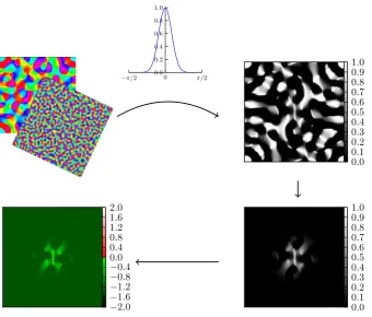
Fig. 4 To construct initial conditions from artificially generated pinwheel maps, we first took such a pinwheel map with a certainscaling(upper left), then we chose a selection of excited orientations by means of a Gaussian. The width of the Gaussian gives the selectiondepth(upper right). After that, we masked the result spatially with another Gaussian distribution that is radially symmetric (lower right). The width of this Gaussian gives the third parameter, thesizeof the pattern. Finally the result is scaled, giving rise to the fourth parameter, we called theexcessand added to the activator variable in the homogeneous state (lower left). The inhibitor variable is put into the homogeneous state
allows us to achieve this aim easily. In order to attack this problem, we turned to the physiological motivation of the chosen model explained in Sect.2.
A set of initial conditions should naturally reflect plausible spatial perturbations of the homogeneous steady state of the cortex. This can be achieved by defining local-ized but spatially structured activity states on large scales of the order of millimeters. Such pattern are obtained from cortical feature maps (see Fig.4) by sampling three parameters (scaling,depth, andsize) that define patches of lateral coupling in theses maps. A fourth parameter (excess) determines the amplitude of the perturbation. In the following, we first describe the rational behind using a cortical feature map and then the sampling.
3.3.1 Rational to Use Cortical Feature Map
region to process visual information from the eyes. Migraine aura symptoms often start there or nearby where similar feature maps exist.
In V1, neurons within vertical columns (through the cortical layers) represent by their activity patterns edges, elongated contours, and whole textures “seen” in the vi-sual field. This representation has a distinct periodically microstructured pattern: the pinwheel map. Neurons preferentially fire for edges with a given orientation and the preference changes continuously as a function of cortical location, except at singu-larities, the pinwheel centers, where the all the different orientations meet [36,37].
Iso-orientation domains form continuous bands or patches around pinwheels and, on average, a region of about 1 mm2(hypercolumn) will contain all possible orienta-tion preferences. This topographical arrangement allows one hypercolumn to analyze all orientations coming from a small area in the visual field, but as a consequence, the cortical representation of continuous contours in the visual field is depicted in a patchy, discontinuous fashion [38]. In general, spatially separated elements are bound together by short- and long-range lateral connections. While the strength of the local short-range connection within one hypercolum is a graded function of cortical dis-tance, mostly independent of relative orientation [39], long-range connections over several hypercolumns connect only iso-orientation domains of similar orientation preference [40,41]. Even nearby regions, which are directly excitatory connected, have an inhibitory component through local inhibitory interneurons and this is likely be used to analyze angular visual features such as corners or T junctions [39].
Given the arguments above, we can now obtain localized yet spatially structured activity states on the scale we aim for as initial conditions by using iso-orientation domains that form continuous patches around pinwheels and extend in a discontinu-ous fashion over larger areas. In these patches, neural activity can get into a critical mode, like neural avalanches [42] that would locally perturb the ionic homeostasis as exemplary shown in Fig.5(lower left).
3.3.2 Sampling of Patterns in Cortical Feature Maps
In [43], the authors analyzed the design principles that lie behind the columnar or-ganization of the visual cortex. The precise design principles of this cortical organi-zation is governed by an annulus-like spectral structure in Fourier domain [36,43], which is determined by mainly one parameter (scaling), that is, the annulus width. The parameter depthreflects the tuning properties of orientation preference or we can also interpret this as the range of orientation angles that we consider within the iso-orientation domain. The third parameter reflects the distance long-range coupling ranges before it significantly attenuates.
These design principles can be exploited and a procedure can be designed to con-struct maps with the same properties. The concon-structed maps come very close to the maps found in brains of macaque monkeys (see [43] and references therein).
Fig. 5 An example of a transient solution. Initial conditions, i.e., activator concentrationuat 0 sec (upper left), snapshot of activator-concentrationuafter 30 sec (upper right), after 180 sec (lower right). Time of passing through threshold valueu0=0 from below the first time, i.e., passing of the wave front (lower
left)
by means of a Gaussian, we choose a range of orientations that is excited. Math-ematically speaking, this is the concatenation of the Gaussian distribution with the pinwheel map. This gives the next parameter, namely the width of the Gaussian that selects the angles, we call that parameter thedepth. The next step is to constrain the generated pattern spatially by multiplication with another Gaussian, which is defined on the planeP and chosen to be rotationally symmetric. The width of this Gaussian gives rise to the third parameter, thesizeof the pattern. Finally, we multiply the pat-tern by a certain amplitude, which is chosen such that the integral of the patpat-tern over the plane gives a chosen number, which constitutes the fourth parameter, we called theexcess.
activity like in neural avalanche, to the activator variableu, which represents the ionic imbalance most notably the extracellular potassium concentration.
In a first run, we scanned the space spanned by the four parameters coarsely. We used the marginal distributions of the number of solutions with an excitation dura-tion (ED)>0 with respect to the parameters to decide how densely to sample the parameter space in the final run.
4 Statistical Properties of Transient Localized Waves
To explore the typical transient patterns that the system described by Eqs. (1)–(3) generates, we want to know how the system responds to the initial conditions as de-scribed before. In characterizing the transient solutions, the same problem we had to obtain equally space initial conditions arises when appropriate characteristic param-eters for the solutions have to be defined.
To explain the three parameters, we have chosen to characterize the solutions and why they suit this problem, it is helpful to have a look at the lower left part of Fig.5, in which an example solution is displayed. The first parameter we chose is the maximal area in which such a solution has activator concentration over a certain threshold level at one instant of time, termed maximal instantaneous area (MIA). The threshold level is taken to beu=0, although this is the same threshold as used foru0to define
S, this is rather convenience than necessity. The second parameter is the total area that has experienced an activator concentration above this level at some time during the course of the solution, termed total affected area (TAA). The third parameter is the time, during which the area of activator concentration above threshold is nonzero, termed the excitation duration (ED). Of course, the exact value of all these parameters for one single solution depends on the choice of threshold. For once, the threshold value has to be chosen such that after the activator concentration has fallen below it; no secondary excitation will be generated.
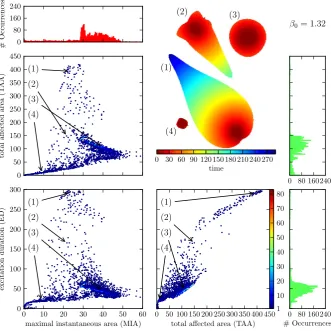
Fig. 6 Distribution of solutions for the control close to∂R
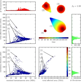
Fig. 7 Distribution of solutions for the control line at an intermediate distance to∂R
When looking at Fig.6, one notices a clustering of the solutions in certain regions of the classification parameters. In the section that depicts the TAA against the MIA, we notice three coarse clusters. Cluster I, the largest with high MIA and compara-tively low TAA; cluster II, one that is less populated with low MIA and low TAA; and cluster III, one that is very sparsely populated with intermediate MIA and high TAA. The boundaries between these clusters are not very sharp. One could think that a solution that affects an overall large area (high TAA) will also affect a large area at one instant of time (high MIA). From looking at the mentioned clusters, one sees that this is not the case, the solutions with the highest MIA have all comparatively low TAA (clusters I and II) and the ones that have a high TAA only achieve an inter-mediate MIA (cluster III).
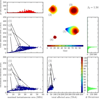
Fig. 8 Distribution of solutions for the control far away from∂R
For these, the area that is affected grows linearly in time because the area that these solutions occupy at one instant of time is constant.
The two clusters I and II that we observed merge to one in this plane of projection because they differ only very little in ED. This can also be noted when comparing the planes MIA vs. TAA and MIA vs. ED; also here, the cluster III with high TAA translates to a cluster with high ED and the cluster I with high MIA and comparatively low TAA moves closer to cluster II with both low ED and MIA.
When varying theβ0parameter of the control force, the distribution of solutions in MIA–TAA–ED-space changes drastically. Upon raising theβ0 parameter from
β0=1.32 overβ0=1.33 toβ0=1.34, the system is put more and more into the subexcitable regime and the solutions are less and less affected by the ghost behavior (saddle-node bifurcation); see Fig.3. This is noticeable by observing that the cluster with high TAA/high ED becomes less pronounced and vanishes almost completely for β0=1.34. This can be understood as an interplay between the mean value of MIA in cluster III at about 25 andS at the propagation boundary (at∂P,S≈24,
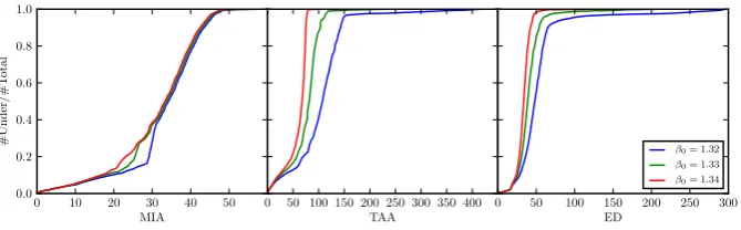
Fig. 9 Cumulative distribution functions for the different classification parameters
the control line farthest away from the saddle-node bifurcation (β0=1.34),∂P is below even the smallest values of MIA in cluster III. Note that the value ofS at the ghost is about 6, well below the propagation boundary. Also, the other two clusters merge though there still exist solutions with high and with low MIA, but the transition is much more fuzzy than it was before.
In Figs.6,7, and 8, we have included a little “bestiary” to illustrate the typical courses of solutions in the respective clusters and their change upon varying the pa-rameterβ0, the initial conditions for solutions 1–4 in these figures are always the same. From this arbitrarily chosen selection, we see that the MIA of each solution hardly changes between theβ0values, whereas the change of TAA and ED always go hand in hand and—depending on the cluster—can be up to four-fold for the chosen range ofβ0.
One could argue that the formation of clusters is an artefact of the choice of initial conditions. There is no simple answer to this. As mentioned, it is not possible to examine the complete set of initial conditions. Neither does this set carry a helpful structure which would allow a sensible “equidistant” sampling. This is the reason why we made the mentioned choice of initial conditions. For testing purposes, we also tried different schemes for the generation of initial conditions and found the same distribution of clusters qualitatively.
In Fig.9, we have plotted the cumulative distribution functions for the three clas-sification parameters and the three choices of mean field control. From this picture, we see that the distribution of the MIA is hardly influenced by the choice of control. This is very different for TAA and ED. For the TAA, for example, there are values (around 75), where for one choice of control the majority of solutions is below and for another choice the majority is above. For example, the fraction of values below TAA=80 is 0.995 forβ0=1.34 and 0.216 forβ0=1.32. Also, we see that the cu-mulative distribution function for the TAA converges to 1 much slower, the closer the control is to the saddle-node bifurcation. This means that more solutions with high TAA exist for these choices of control.
5 Discussion
of this canonical model. Secondly, the possible congruence between the prevalence of migraine subforms with the statistical properties of the wave patterns we observed is discussed. Thirdly, we end with a brief outlook on novel therapeutic approaches in episodic migraine based on the here suggested pattern forming processes.
5.1 Canonical Model and Free Parameters for Weakly Excitable Media
Central to our approach is the localization resp. spatial confinement of the transient traveling waves. Reaction-diffusion waves would engulf all of the medium, if formed in a two-variable system with only one activator and one inhibitor with the system’s parameters in the appropriate regime. In contrast, localized traveling waves indicate a demand-controlled excitability. Similar ideas to obtain localized traveling, though not transient, waves have been introduced in various contexts, for instance, an integral negative feedback or a third, fast diffusing inhibitory component for moving spots in semiconductor materials, gas discharge phenomena, and chemical systems [31,44– 46]. Furthermore, in neural field models [47], localized two-dimensional bumps are studied [48–50] in integrodifferential equations (without diffusion) in the context, for example, of memory formation [51]. Localized structures have also been discussed in the context of cortical spreading depression (SD) in migraine before, in particular a model with narrowly tuned parameters that shows transient waves [13,52,53] and a model with mean field feedback control that allows for localized waves [30]. But it is for the first time now that a model is presented in which wave phenomena oc-cur that are both localized and transient, so that a variety of new questions that are controversially discussed in migraine research [18,54–56] can be addressed. A cen-tral question is of course, which level of detail a model of SD needs to investigate localization of SD and the transient response properties.
Physiological detailed models of SD are given by conductance-ion-based mod-els with 9 to 29 dynamical variables in various (∼200) electrically coupled neural compartments [57–59]. They usually do not include lateral space—the compartments extend in the vertical direction to model the apical dendritic tree, that is, these mod-els are not spatially extended to describe an excitable medium. In fact, this lateral extension is far from straightforward. Naively adding diffusion to the extracellular dynamical ion concentrations is possible but does not reflect the necessary detail that needs to be considered to take the spatial continuum limit. Neural field models, for example, describe this limit [47]. The first part of the global inhibitory feedback by neurovascular coupling, i.e., the fast spread of neural hyperactivity that initiates hypermia—as we suggested in this study—can be modeled by neural fields. The sec-ond part of this neurovascular coupling, the actual feedback signal needs also some physiological detail. This cannot easily be incorporated because neural field models are rate-based or activity-based while the detailed SD models [57–59] start with a conductance-based Hodgkin–Huxley approach and include ion-based dynamics but do not describe the dynamics on a rate-based foundation.
several centimeters and on a temporal scale of up to one hour. Quite apart from the fact that five orders of magnitude in both the spatial and temporal scales suggest that the macroscopic phenomena require their own level of description in some form of effective medium theory.
We suggested that the primary objective in research relating SD to migraine should be to obtain a measure of the noxious signatures that are transmitted into the meninges during SD [60,61]. Canonical reaction-diffusion models seem to be at least one way to approach this objective. A further advantage of such canonical models lies in the fact that they allow insight in the phase space structure of the whole class of models they represent, as schematically shown in Fig.1. Therefore, in the following, we will argue in which sense our model is canonical for the problem we attack.
Generally speaking, an excitable medium is a spatially extended system with a stable homogeneous steady state being the quiescent state and one or many excited states that develop after a sufficient perturbation from the quiescent state (Fig.1a). The excited states are traveling wave solutions that propagate with a stable profile of permanent shape (possibly with some temporal modulation, such as breathing or me-andering). To study generic features of an excitable medium, the simulations are often carried out in the reaction-diffusion system given by Eqs. (1), the popular FitzHugh– Nagumo kinetics. Originally, the FitzHugh–Nagumo kinetics were a caricature of the electrophysiological properties of excitable membranes [62,63], but these equations withD=0 became a canonical model oflocalexcitability of type II (based on Hopf bifurcation, either supercritical with subsequent extremely fast transition to a large amplitude limit cycle, named canard explosion [64], or subcritical [65]). ForD=0, the FitzHugh–Nagumo kinetics became also a canonical model forspatialexcitability [32]. Sometimes diffusion in the second inhibitory species is included, which we do not consider here. Because we investigate transient behavior originating from a high threshold regime (toward weak excitability), the classification of local excitability in types I and II (based on the transition at vanishing threshold, i.e., into the oscillatory regime) is not relevant. Furthermore, it is not clear whether this classification carries over in a meaningful way to the dynamics of spatially extended systems.
We consider the set of Eqs. (1) as canonical for two reasons. First, because theu
(activator) equation of Eq. (1) has the simplest polynomial form of bistability. Note that for this reason this activator equation was originally suggested by Hodgkin and Huxley as the first mathematical model of the potassium dynamics in SD. It was pub-lished by Grafstein, who also provided experimental data supporting such a simple reaction-diffusion scheme for the front dynamics in SD [66]. Second, the inhibitor equation of Eq. (1) has a linear rate function, in fact, the rate function is only a func-tion of the activatoru. This is the simplest inhibitor dynamics needed for pulse prop-agation. By neglecting an additional linear term−γ v in the inhibitor rate function, we limit the origin of excitability to the case of a supercritical Hopf bifurcation with subsequent canard explosion and avoid the bistable regime that exits in the subcrit-ical case. The subcritsubcrit-ical Hopf bifurcation occurs only in a narrow regime whenγ
is close to 1 andβ close to 0. We have tested some simulations withγ =0.5 with similar results.
ε, the time scale separation of activator and inhibitor dynamics. Of course, the choice of parameters can be quite different, a common choice isαin the cubic rate function
f (u)=u(u−α)(u−α)but there are only two free parameters or two equivalent groups of parameters. So, there are the same bifurcations in the parameter planes
(ε, β)or (ε, α), but to map the dynamics between equivalent groups of parameters might involve changes in time, space, and concentrations scales.
In particular, the question of how the incidence of MA is reflected in the distance to the saddle-node bifurcation, involves a measure on the parameter space whether is(ε, β),(ε, α), or any other parameter plane. We have previously suggested to get such measures from pharmacokinetic-pharmacodynamic models [53].
5.2 Application to Migraine Pathophysiology
We suggest a qualitative congruence between the prevalence of MO and MA with the statistical properties we found in the transient response properties. We do not suggest that all migraine attacks are related to SD nor that pain formation in MA is exclusively caused by SD. Rather that SD is one pathway of pain formation in both symptom-based subtypes MO and MA. We refer to this pathway as the “spreading depression”-theory of migraine [17]. The “migraine generator”-theory (MG) is for various reasons not less plausible [54]. It assumes a dysfunction in a central pattern generator in the brainstem that modulates the perception of pain. Some of the seem-ingly conflicting and controversially discussed evidence is probably resolved when one considered the basis of the classification of migraine subforms. We currently have a symptom-based classification for migraine with possibly overlapping etiologies for individual subforms. In the light of an etiology-based classification with possibly overlapping symptoms the conflicts seem less puzzling to us. To further resolve this, we investigated the interplay of SD and MG and suggested to unify these approaches within a network theory [61].
In the remainder of this section, we focus first on migraine pain and then on the migraine aura.
5.2.1 Migraine Pain
Fig. 10 Schematic representation of cross section of cortex, meninges, and skull. The leptomeninges refer to the pia mater and arachnoid membrane. SD releases noxious substances with increased blood flow thought to diffuse outward. Activation of pain pathways can depend on MIA
If diffusion vertical to the affected cortical area is critical, size and shape of this area should play a critical role; see Fig.10. This suggests that SD waves activate nociceptive mechanisms dependent upon a sufficiently large instantaneously affected cortical area, i.e., large MIA and, as stated before, the primary objective should be to obtain a measure of the noxious signatures that are transmitted into the meninges during SD.
5.2.2 Migraine Aura
Fig. 11 Statistical analysis of output data. For allfour pictures, we took all data points with MIA in the interval[MIAlow,MIAlow+10](“sliding window”) and analyzed the connection with TAA (left column)
and ED (right column). In theupper row, the average value is plotted withsolid lines; the area of one standard deviation around this value isshaded. In thelower row, the correlation coefficient between MIA and the respective quantity is plotted. In all plots, thedotted linesindicates the number of events for the respective interval with MIAlow
The connection between MIA and TAA as well as MIA and ED in our model is shown in Fig.11. It shows that in the range of high MIA the average values for TAA and ED are becoming smaller. From Fig.11, we can also read off that the range with the most events is in the regime of relatively high MIA (around 30) and signifi-cantly after the peak of ED resp. TAA. Moreover, in the range with most events, the correlation coefficient r(MIA,ED)is always negative and the correlation coefficient r(MIA,TAA)is mostly negative. All these effects are stronger, the closer the control line is located to the saddle-node bifurcation.
From these statistical correlations between MIA and TAA resp. ED and the distri-bution of the number of events, one could speculate that cases of MA are more rare and the quality of the headache in these cases might be less severe. This is exactly what has been reported in the medical literature [73].
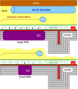
Fig. 12 Development of SD and model-based control. SD based on a two-variable reaction-diffusion mechanism engulfs all the densely packed excitable neurons in the cortex (top row). The activator con-centration is inred, the inhibitor inyellowin this schematic illustration. Long-range inhibitory feedback (green) is a well-established pattern formation mechanism to confine the spread (bottom row). The pre-dicted emerging transient patterns offer a model-based analysis of phase-depended stimulation protocols. In the classical paradigm, applying noninvasive neuromodulation devices, which may succeed to block SD locally (c), would result in a reentrant pattern (d). In the new paradigm of localized SD waves that we suggest, a phase-dependent stimulation protocol might target intelligently with noise the bottle-neck passage (g) (see main text), while a different protocol might be considered during the initial nucleation phase (e)
5.3 Model-Based Control by Neuromodulation
We briefly discuss model-based control and means by which neuromodulation tech-niques may affect pathways of pain formation and the aura phase.
The emerging transient patterns and their classification according to size and dura-tion offer a model-based analysis of phase-dependent stimuladura-tion protocols for non-invasive neuromodulation devices, e.g., utilizing transcranial magnetic stimulation (TMS) [74], to intelligently target migraine. For instance, noise is a very effective method to drive the system back into the homogeneous steady state more quickly; see Fig.12. In general, responses of nonlinear systems to noise applied when the system is just before or past a saddle-node bifurcation are well studied. Before the saddle-node on limit cycle bifurcation, the phenomenon of coherence resonance (CR) describes that a certain amount of noise makes responses most coherent [75]. Behind the saddle-node bifurcation on a limit cycle, the time the flows spend in the bottleneck region of the ghost is shortened [76]. However, noise would, according to our model, mainly positively affect ED and TAA, that is, the aura, while it could even worsen the headache, if applied early during the nucleation and growth process. Therefore, TMS with noise stimulation protocols, which are currently investigated, should be applied only some time after first noticing aura symptoms.
propitious to propose fusing control theory with neural stimulation for the treatment of dynamical brain disease.”
We suggest to consider migraine as a dynamical disease that could benefit from model-based control therapies.
Competing Interests
The authors declare no conflicts of interest.
Authors’ Contributions
MAD conceived the model and its application to migraine aura. TMI implemented the simulation. MAD and TMI analysed the mathematical model, interpreted the results, wrote the paper, and read and approved the final manuscript.
Acknowledgements The authors kindly acknowledge the support from the Deutsche Forschungs-gemeinschaft (DFG) in the frameworks of SFB910 and GRK1558, and from the Bundesministerium für Bildung und Forschung (BMBF 01GQ1109). This research (MD) has been supported in part also by the Mathematical Biosciences Institute at the Ohio State University and the National Science Foundation under Grant No. DMS 0931642. The authors would also like to thank Gerold Baier, Michael Guevara, Zachary Kilpatrick, and Eckehard Schöll for helpful discussions and advice.
References
1. Hodgkin AL:The local electric changes associated with repetitive action in a medullated axon.
J Physiol1948,107:165.
2. Hodgkin AL, Huxley AF:A quantitative description of membrane current and its application to conduction and excitation in nerve.J Physiol1952,117:500.
3. van der Pol B:On relaxation oscillations.Philos Mag1926,2:978-992.
4. Bonhoeffer KF:Modelle der Nervenerregung.Naturwissenschaften1953,40(11):301-311. 5. FitzHugh R:Mathematical models of excitation and propagation in nerve. InBiological
Engi-neering. Edited by Schwan HP. New York: McGraw-Hill; 1969:1-85.
6. Rinzel J, Ermentrout GB:Analysis of neural excitability and oscillations. InMethods in Neuronal Modeling. Edited by Koch C, Segev I. Cambridge: MIT Press; 1989:251-291.
7. Izhikevich EM:Neural excitability, spiking, and bursting.Int J Bifurc Chaos2000,10:1171-1266. 8. Keener JP, Sneyd J:Mathematical Physiology. New York: Springer; 1998.
9. Kapral R, Showalter K (Eds):Chemical Waves and Patterns. Dordrecht: Kluwer; 1995. 10. Schöll E:Nonequilibrium Phase Transitions in Semiconductors. Berlin: Springer; 1987.
11. Dahlem MA, Engelmann R, Löwel S, Müller SC:Does the migraine aura reflect cortical organi-zation.Eur J Neurosci2000,12:767-770.
12. Hadjikhani N, Sanchez Del Rio M, Wu O, Schwartz D, Bakker D, Fischl B, Kwong KK, Cutrer FM, Rosen BR, Tootell RB, Sorensen AG, Moskowitz MA:Mechanisms of migraine aura revealed by functional MRI in human visual cortex.Proc Natl Acad Sci USA2001,98:4687-4692.
13. Dahlem MA, Hadjikhani N:Migraine aura: retracting particle-like waves in weakly susceptible cortex.PLoS ONE2009,4:e5007.
14. Goadsby PJ, Lipton RB, Ferrari MD:Migraine—current understanding and treatment.N Engl J Med2002,346:257-270.
15. Leão AAP, Morison RS:Propagation of cortical spreading depression.J Neurophysiol1945, 1:33-45.
17. Lauritzen M:Cortical spreading depression as a putative migraine mechanism.Trends Neurosci
1987,10:8-13.
18. Ayata C:Cortical spreading depression triggers migraine attack: pro.Headache2010, 50(4):725-730.
19. Eikermann-Haerter K, Ayata C:Cortical spreading depression and migraine.Curr Neurol Neurosci Rep2010,10(3):167-173.
20. Hansen JM, Lipton RB, Dodick DW, Silberstein SD, Saper JR, Aurora SK, Goadsby PJ, Charles A: Migraine headache is present in the aura phase: a prospective study. Neurology 2012, 79(20):2044-2049.
21. Viana M, Sprenger T, Andelova M, Goadsby PJ:The typical duration of migraine aura: a system-atic review.Cephalalgia2013,33:483-490.
22. Woods RP, Iacoboni M, Mazziotta JC:Brief report: bilateral spreading cerebral hypoperfusion during spontaneous migraine headache.N Engl J Med1994,331(25):1689-1692.
23. Dreier JP:The role of spreading depression, spreading depolarization and spreading ischemia in neurological disease.Nat Med2011,17:439-447.
24. Herreras O, Largo C, Ibarz JM, Somjen GG, Martin del Rio R:Role of neuronal synchronizing mechanisms in the propagation of spreading depression in the in vivo hippocampus.J Neurosci
1994,14:7087-7098.
25. Wilkinson F:Auras and other hallucinations: windows on the visual brain.Prog Brain Res2004, 144:305-320.
26. Izhikevich EM, FitzHugh RA:FitzHugh–Nagumo model.Scholarpedia2006,1(9):1349.
27. Craster RV, Sassi R:Spectral algorithms for reaction-diffusion equations.Technical report 99, 2006.
28. Mikhailov AS:Foundations of Synergetics.Volume I. Berlin: Springer; 1990.
29. Dahlem MA, Schneider FM, Schöll E:Failure of feedback as a putative common mechanism of spreading depolarizations in migraine and stroke.Chaos2008,18:026110.
30. Dahlem MA, Graf R, Strong AJ, Dreier JP, Dahlem YA, Sieber M, Hanke W, Podoll K, Schöll E: Two-dimensional wave patterns of spreading depolarization: retracting, re-entrant, and stationary waves.Physica D2010,239:889-903.
31. Krischer K, Mikhailov AS:Bifurcation to traveling spots in reaction-diffusion systems.Phys Rev Lett1994,73(23):3165-3168.
32. Winfree AT:Varieties of spiral wave behaviour: an experimentalist’s approach to the theory of excitable media.Chaos1991,1:303-334.
33. Mikhailov AS, Zykov VS:Kinematical theory of spiral waves in excitable media: comparison with numerical simulations.Physica D1991,52:379-397.
34. Hakim A, Karma V:Theory of spiral wave dynamics in weakly excitable media: asymptotic re-duction to a kinematic model and applications.Phys Rev E1999,60:5073-5105.
35. Krupa M, Sandstede B, Szmolyan P:Fast and slow waves in the FitzHugh–Nagumo equation.
J Differ Equ1997,133:49-97.
36. Rojer AS, Schwartz EL:Cat and monkey cortical columnar patterns modeled by bandpass-filtered 2D white noise.Biol Cybern1990,62(5):381-391.
37. Bonhoeffer T, Grinvald A:Iso-orientation domains in cat visual cortex are arranged in pinwheel-like patterns.Nature1991,353:429-431.
38. Eysel U:Turning a corner in vision research.Nature1999,399(6737):643-644.
39. Das A, Gilbert CD:Topography of contextual modulations mediated by short-range interactions in primary visual cortex.Nature1999,399(6737):655-661.
40. Gilbert CD:Horizontal integration and cortical dynamics.Neuron1992,9:1-13.
41. Gilbert CD, Das A, Ito M, Kapadia M, Westheimer G:Spatial integration and cortical dynamics.
Proc Natl Acad Sci USA1996,93(2):615-622.
42. Beggs JM, Plenz D:Neuronal avalanches in neocortical circuits.J Neurosci2003, 23(35):11167-11177.
43. Niebur E, Wörgötter F:Design principles of columnar organization in visual cortex.Neural Com-put1994,6:602-613.
44. Ohta T, Mimura M, Kobayashi R:Higher-dimensional localized patterns in excitable media. Phys-ica D1989,34(1–2):115-144.
45. Schenk CP, Or-Guil M, Bode M, Purwins HG:Interacting pulses in three-component reaction-diffusion systems on two-dimensional domains.Phys Rev Lett1997,78:3781.
47. Bressloff PC:Spatiotemporal dynamics of continuum neural fields.J Phys A2012,45(3):033001. 48. Lu Y, Sato Y, Amari S:Traveling bumps and their collisions in a two-dimensional neural field.
Neural Comput2011,23(5):1248-1260.
49. Bressloff P, Kilpatrick Z:Two-dimensional bumps in piecewise smooth neural fields with synaptic depression.SIAM J Appl Math2011,71(2):379-408.
50. Coombes S, Schmidt H, Bojak I:Interface dynamics in planar neural field models.J Math Neurosci
2012,2:9.
51. Kilpatrick ZP, Bard Ermentrout G:Wandering bumps in stochastic neural fields.SIAM J Appl Dyn Syst2013,12:61-94.
52. Dahlem MA, Müller SC:Migraine aura dynamics after reverse retinotopic mapping of weak excitation waves in the primary visual cortex.Biol Cybern2003,88:419-424.
53. Dahlem MA, Schneider FM, Schöll E:Efficient control of transient wave forms to prevent spread-ing depolarizations.J Theor Biol2008,251:202-209.
54. Akerman S, Holland PR, Goadsby PJ:Diencephalic and brainstem mechanisms in migraine.Nat Rev, Neurosci2011,12(10):570-584.
55. Fioravanti B, Kasasbeh A, Edelmayer R, Skinner DP, Hartings JA, Burklund RD, De Felice M, French ED, Dussor GO, Dodick DW, Porreca F, Vanderah TW:Evaluation of cutaneous allodynia following induction of cortical spreading depression in freely moving rats.Cephalalgia2011, 31(10):1090-1100.
56. Levy D, Moskowitz MA, Noseda R, Burstein R:Activation of the migraine pain pathway by cor-tical spreading depression: do we need more evidence?Cephalalgia2012,32(7):581-582. 57. Kager H, Wadman WJ, Somjen GG:Simulated seizures and spreading depression in a neuron
model incorporating interstitial space and ion concentrations.J Neurophysiol2000,84:495-512. 58. Shapiro BE:Osmotic forces and gap junctions in spreading depression: a computational model.
J Comput Neurosci2001,10:99-120.
59. Miura RM, Huang H, Wylie JJ:Cortical spreading depression: an enigma.Eur Phys J Spec Top
2007,147:287-302.
60. Karatas H, Erdener SE, Gursoy-Ozdemir Y, Lule S, Eren-Kocak E, Sen ZD, Dalkara T: Spread-ing depression triggers headache by activatSpread-ing neuronal Panx1 channels. Science 2013, 339(6123):1092-1095.
61. Dahlem MA:Migraine generator network and spreading depression dynamics as neuromodula-tion targets in episodic migraine.arXiv:1303.2256, 2013.
62. FitzHugh R:Impulses and physiological states in theoretical models of nerve membrane.Biophys J1961,1:445-466.
63. Nagumo J, Arimoto S, Yoshizawa S:An active pulse transmission line simulating nerve axon.Proc IRE1962,50:2061-2070.
64. Wechselberger M:Existence and bifurcation of canards inR3in the case of a folded node.SIAM J Appl Dyn Syst2005,4:101-139.
65. Ermentrout GB:Neural networks as spatio-temporal pattern-forming systems.Rep Prog Phys
1998,61:353-430.
66. Grafstein B:Neural release of potassium during spreading depression. InBrain Function. Cortical Excitability and Steady Potentials. Edited by Brazier MAB. Berkeley: University of California Press; 1963:87-124.
67. Moskowitz MA, Nozaki K, Kraig RP:Neocortical spreading depression provokes the expression of c-fos protein-like immunoreactivity within trigeminal nucleus caudalis via trigeminovascular mechanisms.J Neurosci1993,13(3):1167-1177.
68. Bolay H, Reuter U, Dunn AK, Huang Z, Boas DA, Moskowitz MA:Intrinsic brain activity triggers trigeminal meningeal afferents in a migraine model.Nat Med2002,8(2):136-142.
69. Ingvardsen BK, Laursen H, Olsen UB, Hansen AJ:Possible mechanism of c-fos expression in trigeminal nucleus caudalis following cortical spreading depression.Pain1997,72(3):407-415. 70. Moskowitz MA, Kraig R:Comment on Ingvardsen et al., PAIN, 72 (1997) 407-415.Pain1998,
76(1-2):265-267.
71. Zhang X, Levy D, Noseda R, Kainz V, Jakubowski M, Burstein R:Activation of meningeal noci-ceptors by cortical spreading depression: implications for migraine with aura.J Neurosci2010, 30(26):8807-8814.
72. Tfelt-Hansen PC:Permeability of dura mater: a possible link between cortical spreading depres-sion and migraine pain? A comment.J Headache Pain2011,12:3-4.
74. Lipton RB, Dodick DW, Silberstein SD, Saper JR, Aurora SK, Pearlman SH, Fischell RE, Ruppel PL, Goadsby PJ:Single-pulse transcranial magnetic stimulation for acute treatment of migraine with aura: a randomised, double-blind, parallel-group, sham-controlled trial.Lancet Neurol2010, 9:373-380.
75. Lindner B, García-Ojalvo J, Neiman A, Schimansky-Geier L:Effects of noise in excitable systems.
Phys Rep2004,392:321-424.
76. Strogatz SH:Nonlinear Dynamics and Chaos. Cambridge: Westview Press; 1994.
77. Silberstein SD, Dodick DW, Saper J, Huh B, Slavin KV, Sharan A, Reed K, Narouze S, Mogilner A, Goldstein J, Trentman T, Vaisma J, Ordia J, Weber P, Deer T, Levy R, Diaz RL, Washburn SN, Mekhail N:Safety and efficacy of peripheral nerve stimulation of the occipital nerves for the management of chronic migraine: results from a randomized, multicenter, double-blinded, con-trolled study.Cephalalgia2012,32:1165-1179.
78. Diener HC:Occipital nerve stimulation for chronic migraine: already advised?Cephalalgia2012, 32:1163-1164.
79. Baier G, Goodfellow M, Taylor PN, Wang Y, Garry DJ:The importance of modeling epileptic seizure dynamics as spatio-temporal patterns.Front Physiol2012,3:281.