Conference Paper
1
Simulation and Optimization of Control
2
of Selected Phases of Gyroplane Flight
3
Wienczyslaw Stalewski 1*
4
1 Institute of Aviation, Al. Krakowska 110/114, Warszawa, Poland; [email protected]
5
* Correspondence: [email protected]; Tel.: +48-888-146-748
6
Abstract: The optimization methods are increasingly used to solve challenging problems of
7
aeronautical engineering. Typically, the optimization methods are utilized in design of aircraft
8
airframe or its structure. The presented study is focused on an improvement of
9
aircraft-flight-control procedures through the numerical optimization approach. The optimization
10
problems concern selected phases of flight of light gyroplane - a rotorcraft using an unpowered
11
rotor in autorotation to develop lift and an engine-powered propeller to provide thrust. An original
12
methodology of computational simulation of rotorcraft flight was developed and implemented. In
13
this approach the aircraft-motion equations are solved step-by-step, simultaneously with the
14
solution of the Unsteady Reynolds-Averaged Navier-Stokes equations, which is conducted to
15
assess aerodynamic forces acting on the aircraft. As a numerical optimization method, the BFGS
16
algorithm was adapted. The developed methodology was applied to optimize the flight-control
17
procedures in selected stages of gyroplane flight in direct proximity of the ground, where properly
18
conducted control of the aircraft is critical to ensure flight safety and performance. The results of
19
conducted computational optimizations proved qualitative correctness of the developed
20
methodology. The research results can be helpful in design of easy-to-control gyroplanes and also
21
in the training of pilots of this type of rotorcraft.
22
Keywords: flight simulation; flight control; optimization;CFD; flight dynamics
23
24
1. Introduction
25
Optimization methods are widely considered to be a very effective tool that can significantly
26
improve the performance and exploitation properties of contemporarily designed and constructed
27
aircraft. Typically, the optimization methods are utilized in design of aircraft airframe or its
28
structure that may be optimized simultaneously using a multi-disciplinary approach [1-3]. Fast
29
development of both computational methods and computer hardware offers opportunities to
30
expand the range of applications of optimization methods. As part of this trend, the application of
31
modern computational methods to optimize aircraft-flight-control procedures is presented in this
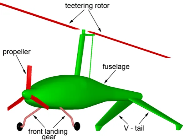
32
paper. The developed methodology for optimization of flight control procedures is discussed on the
33
example of flight of a light gyroplane.
34
A gyroplane is an aerodyne equipped with unpowered main rotor and engine-powered
35
propeller, generating a thrust force necessary to move the aircraft forward. During the gyroplane
36
flight the air flowing around rotating blades of main rotor generates aerodynamic reaction whose
37
vertical component balances the aircraft weight, while the aerodynamic moment is driving the main
38
rotor that rotates in autorotation. However to induce the autorotation phenomenon, the rotor should
39
be initially pre-rotated, which is usually done by the engine driving the propeller. Before the
40
gyroplane loses contact with the ground, the drive of the rotor must be disconnected because this
41
type of rotorcraft does not have any anti-torque devices.
42
Primary flight-control means of gyroplanes are:
43
• longitudinal and lateral tilting of the rotor shaft to ensure a pitch and roll control,
44
• deflections of the rudder to ensure a yaw control.
45
Gyroplanes may be optionally equipped with the following secondary flight controls:
46
• pre-rotator which drives the rotor to initiate its rotation,
47
• changeable collective pitch of rotor blades that may be used for torque reduction in pre-rotation
48
and is necessary to conduct so called "jump takeoff".
49
The classic takeoff of a gyroplane is similar to typical takeoff of an airplane. The gyroplane, with
50
pre-rotated main rotor, starts accelerated run along the runway. The rotor generates more and more
51
thrust. When the thrust exceeds the weight of aircraft, the gyroplane takes off. Gyroplanes usually
52
need short runway to conduct the classic takeoff and they mostly belong to STOL (Short Takeoff and
53
Landing) type of aircraft.
54
In the case of so called “jump takeoff", the gyroplane takes off directly from the ground, without
55
a run along the runway. To perform this maneuver, the rotor head design should allow changing an
56
angle of blade collective pitch during the flight. After initial pre-rotation of the rotor, the drive is
57
disconnected and simultaneously the higher angle of the blade collective pitch is established. The
58
inertia-driven rotor generates high thrust, which makes that the gyroplane jumps upwards. The
59
propeller starts driving the gyroplane in horizontal direction, which makes that the horizontal
60
velocity starts growing and after some time the rotor starts rotating in autorotation, similarly as it is
61
in a case of the classic takeoff.
62
All studies presented in this paper, have been conducted for a gyroplane presented in Figure 1.
63
The gyroplane is equipped with a teetering main rotor, three-bladed tractor-type propeller, front
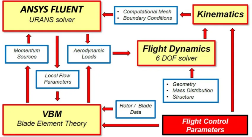
64
landing gear and v-tail that also serves as a rear landing gear. Like in a case of most gyroplanes, the
65
main rotor of the presented gyroplane is characterized by a simple design. It is two-bladed, teetering
66
rotor. Its blades have a rectangular planform, uniform spanwise distribution of airfoil and are not
67
twisted. To enhance the controllability of the gyroplane its rotor-head design enables to control the
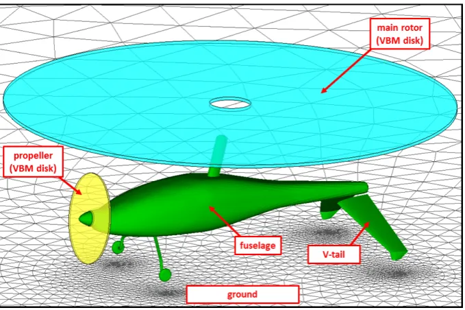
68
collective pitch of rotor blades.
69
Figure 1. Model of the gyroplane being a subject of the research discussed in the paper.
70
An effective and safe takeoff of the gyroplane requires accurate and rapid deflections of
71
flight-control devices. This especially concerns the control of the rotor-pitch angle that has to be
72
changed in time optimally so as to enhance the autorotation effect as much as possible. Additionally,
73
during the jump takeoff, the dynamic changes of the rotor-pitch angle have to be synchronized
74
optimally with dynamic changes of the collective pitch of the rotor blades.
75
The main idea of the presented research was to search for possibly optimal procedures of
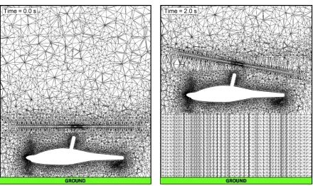
76
control of the gyroplane flight through application of a numerical-optimization methodology. To
77
1. To develop a computational methodology of simulation of a gyroplane flight, especially
79
directed towards high-fidelity simulations of a takeoff and ascent flight of the rotorcraft,
80
2. To develop a numerical-optimization methodology that would be applicable for the solving of
81
problems concerning the optimization of rotorcraft-flight-control procedures,
82
3. To optimize flight-control procedures (i.e. functions describing time-variable settings of the
83
flight-control devices) during the classic takeoff and jump takeoff of the gyroplane, so as to
84
achieve measurable improvement in the aircraft performance in these flight states.
85
Numerical-optimization methods are wider and wider utilized in rotorcraft engineering. Most
86
of them are directed towards optimization of the rotorcraft crucial components such as main rotors
87
or tail rotors. Nowadays, such optimization problems are usually formulated in multidisciplinary
88
form [4]. This includes more and more reliable methods in such areas as Computational Fluid
89
Dynamics (CFD), Computational Structural Mechanics (CSM) or Flight Dynamics. On the other
90
hand, attempts are made to automate the design process itself, by applying numerical optimization
91
methods. The CFD methods have reached sufficient maturity to compute very accurately helicopter
92
rotor aerodynamic performance. The current CFD codes efficiency enables potentially to use them in
93
automatic optimization chains. Such optimization strategies involving URANS (Unsteady
94
Reynolds-Averaged Navier-Stokes) solvers have been applied in aeronautics on fixed wing
95
configurations [5,6] or via adjoint formulation on aircraft configurations [7,8] and have
96
demonstrated their efficiency to be successfully integrated in design cycles. Alternative approaches
97
are based on stochastic-optimization methods (e.g. Genetic Algorithm). Among others, such
98
approach was applied in [3] for optimization of helicopter fuselage (with simulation of main and tail
99
rotor influence) as well as in [1,2] for multidisciplinary optimization of aircraft wings. To cope with
100
extreme complexity of coupling of advanced methods of CFD and numerical-optimization, some
101
authors utilize surrogate models of physical phenomena, as presented in [9,10]. In [11] authors
102
describe an optimization strategy for helicopter rotor blades shape, based on the coupling of an
103
optimization gradient method with a 3D Navier-Stokes solver.
104
Advanced numerical optimization methods coupled with Navier-Stokes solvers, are actually
105
used mostly for an optimization of aircraft external shapes (aerodynamic design) or its structure.
106
In the case of optimization of the rotorcraft flight control procedures, simplified computational
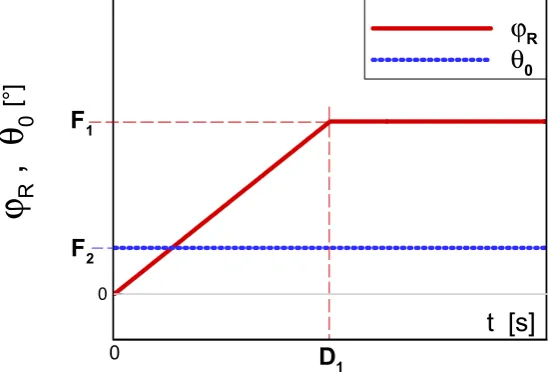
107
models of aircraft aerodynamics are usually used. In particular, it concerns advanced computational
108
tools dedicated for flight-control optimization. Such tools utilize usually simple models of rotorcraft
109
aerodynamics. The aerodynamic effects generated by crucial components of rotorcraft, such as main
110
rotor or tail rotor, are usually modelled using the Lifting-Line Theory or even are based on databases
111
of global aerodynamic characteristics of these rotors. In a case of rotorcraft-flight-control
112
design-and-optimization tool named CONDUIT, the details concerning the utilized both
113
optimization methods and aerodynamic models are discussed thoroughly in references [12,13].
114
In comparison to previously used computational tools supporting the design and optimization
115
of rotorcraft flight control, the approach discussed in this paper is not directly geared to industrial
116
applicability but rather to explore new solutions that could in future be applied in the practice of
117
designing of flight-control systems. The proposed solution distinguishes itself from most of
118
currently utilized approaches by the following assumptions:
119
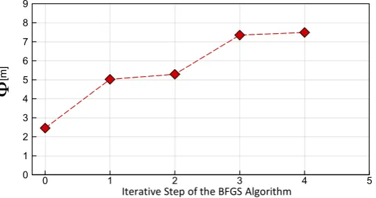
• The rotorcraft-flight-control optimization is based on advanced, gradient-based optimization
120
methods coupled with advanced CFD methods used directly during the rotorcraft-flight
121
simulation for the current determination of aerodynamic loads acting on the aircraft.
122
• The developed methodology is applied to optimize the gyroplane-flight-control procedures
123
(while most of the applications cited in the literature are focused on the optimization
124
of helicopter-flight control).
125
2. Research Methodology
126
The general scheme of the developed methodology of rotorcraft-flight simulation is presented
127
Averaged Navier Stokes) solver ANSYS FLUENT [14]. Flow effects caused by rotating lifting
129
surfaces are modelled by application of the developed UDF (User Defined Function) module Virtual
130
Blade Model (VBM) [3] that is compiled and linked with the essential code of the ANSYS FLUENT
131
software. In the VBM approach, real rotors are replaced by volume discs influencing the flow field
132
similarly as rotating blades. Time-averaged aerodynamic effects of rotating lifting surfaces are
133
modelled by means of artificial momentum source terms placed inside the volume-disc zones placed
134
in regions of activity of real rotors. Such zones, replacing the real rotor and propeller in investigated
135
gyroplane, are shown in Figure 3. The momentum rates, injected from these zones into the fluid, are
136
evaluated based on the Blade Element Theory, associating local flow parameters in rotor-disc zones
137
with aerodynamic characteristics of blade airfoils. Data bases of these characteristics (in general: lift
138
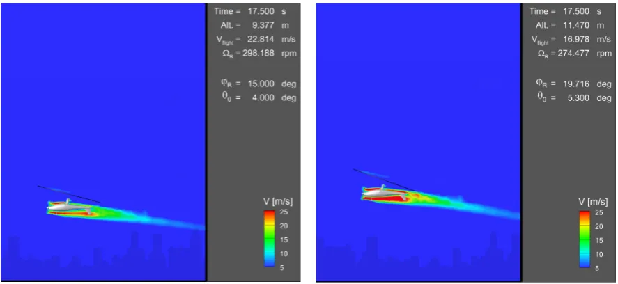
and drag coefficients as functions of angle of attack, for several sets of Mach and Reynolds numbers,
139
similar to those that are expected on the real rotor blades) should be prepared before starting the
140
flight simulation. The original VBM code was significantly modified and expanded by the author of
141
this paper. Beside the essential modules ANSYS FLUENT and VBM, the methodology presented in
142
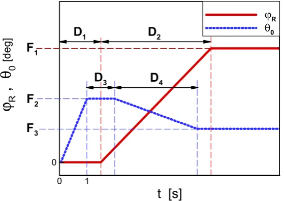
Figure 2 utilizes two additional modules. The module FLIGHT-DYNAMIC gathers information of
143
all momentary loads acting on the rotorcraft and solves 6 degree-of-freedom equations of rotorcraft
144
motion. The module KINEMATICS is responsible for modelling of effects of motion and changes of
145
rotorcraft geometry, which is realized through redefinition of boundary conditions for the ANSYS
146
FLUENT solver and through deformations of computational mesh. The computational model of the
147
gyroplane, shown in Figure 3, was developed so as to enable simulation of flight in proximity of the
148
ground and tilting of the rotor. These motions are realized through appropriate deformations of
149
computational mesh which is done with the use of the Dynamic Mesh technique, implemented in
150
ANSYS FLUENT solver. Examples of such deformations of computational mesh are presented in
151
Figure 4. Additionally, the developed model enables deflecting the gyroplane control surfaces
152
(option not used in the presented study) which is realized through application of Sliding-Mesh and
153
Non-Conformal-Interface techniques implemented in ANSYS FLUENT.
154
Figure 2. General scheme of the developed methodology of rotorcraft-flight simulation.
155
The described complex model of the gyroplane flight was used in optimization studies on
156
flight-control procedures during the gyroplane takeoff. Though the developed methodology enables
157
to solve 6-degree-of-freedom rotorcraft flight dynamics, the presented in the paper simulations were
158
conducted taking into account only 3 degree-of-freedom system, limited to force-balance equations,
159
The method of computational simulation of gyroplane flight, has been applied in optimization
161
studies on flight-control procedures. In these studies, functions describing changes in time of main
162
gyroplane-flight-control means (i.e.: tilt of the main-rotor shaft and collective pitch of rotor blades)
163
have been parameterized. They were uniquely defined by sets of few unknown real numbers - the
164
design parameters. The objective function, considered as a function of unknown design parameters,
165
was defined in presented examples as an altitude which would be achieved by the gyroplane, after
166
reaching the assumed distance from the takeoff point. The optimization problem consisted in
167
searching for the set of the design parameters that would maximize the objective function.
168
Figure 3. Computational model of the gyroplane flying in proximity of the ground.
169
To solve the defined above optimization problem, the appropriately adapted BFGS
170
Algorithm [5] has been applied. The method BFGS, named after C.G. Broyden, R. Fletcher,
171
D. Goldfarb and D. Shanno, belongs to quasi-Newton methods - a class of hill-climbing optimization
172
techniques that seek a stationary point of a given objective function (preferably twice continuously
173
differentiable). Gradient-based methods utilize a necessary condition for optimality, saying that at
174
optimum point the gradient of objective function is a zero vector. Usually such methods do not
175
guarantee the convergence to the exact optimum, unless the objective function has a quadratic
176
Taylor expansion near an optimum. However, BFGS Algorithm has proven to have good
177
performance even in such case when the objective functions were not smooth.
178
In quasi-Newton methods, including the BFGS Algorithm, the Hessian matrix of second
179
derivatives does not need to be evaluated directly. Instead, the Hessian matrix is approximated
180
using updates specified by gradient evaluations or approximate gradient evaluations. The latter
181
approach has been applied in the presented optimization studies.
182
Like in all cases of gradient-based methods, the optimal solution has been searched for, in
183
sequential iterative steps. In each step, the components of the gradient vector (partial derivatives of
184
the objective function with respect to the unknown design parameters) were evaluated by means of
185
one-sided finite-difference approximation. In the presented approach, this required performing at
186
least N+1 simulations of the gyroplane flight, where N was the number of the independent variables
187
(design parameters). In addition, solving the typical for the BFGS method the auxiliary
188
one-dimensional problem of finding the optimal movement in the newfound search direction,
189
several additional simulations of gyroplane flight was conducted at each sequential step of the
190
optimization process.
191
It should be mentioned, that the BFGS method has been developed also in a variant with simple
192
box constraints [16] and usually such variant of the method has been applied in the presented
193
Figure 4. Cross-section of computational mesh around the gyroplane in two different stages of flight
195
Left side: a ground pre-rotation, right side: a forward flight few meters above the ground.
196
3. Optimization of Gyroplane-Takeoff-Control Procedures
197
The presented below two examples of conducted numerical optimizations of
198
gyroplane-flight-control procedures concern the described above two types of takeoff of the
199
gyroplane: classic takeoff and jump takeoff. In both cases, the optimization process aimed at
200
maximization of the altitude reached by the gyroplane after traveling certain distance from the
201
takeoff place. The both optimizations were conducted for the same assumed general flight
202
conditions:
203
• total mass of the gyroplane: 600 kg,
204
• maximum thrust of the propeller: 2943 N.
205
3.1. Classic Takeoff of the Gyroplane
206
The optimization of classic-takeoff-control procedure has been conducted in respect to
207
time-variable pitch angle of main rotor (ϕR), which was considered as the only flight control
208
parameter. The angle of collective pitch of rotor blades (θ0), unchangeable during the flight, has been
209
assumed as additional unknown parameter. Based on these assumptions, the flight control
210
procedure during the classic takeoff has been defined by graphs presented in Figure 5, where:
211
• function ϕR(t) is uniquely defined by unknown parameters D1 and F1,
212
• constant function θ0(t) = const. is uniquely defined by unknown parameter F2.
213
In this case, the optimization problem consisted in determination of optimal values of unknown
214
parameters D1, F1 and F2. The optimization aimed at maximization of the altitude (H) reached by the
215
gyroplane after traveling the distance X=200 m from the takeoff place, which is explained in Figure 6.
216
The optimization problem was formulated in mathematical terms as a search for the set of the design
217
parameters D1, F1 and F2 maximizing the following function Φ:
218
Φ(D1, F1, F2) = H(X=200m), (1)
taking into account the following constraints:
219
F2 ≤θ0max , (3)
| F1/D1 | ≤λ1, (4)
F1≤ϕRmax , (5)
where: λ1 - limit of angular speed of change of ϕR, ϕRmax - maximum of rotor pitch and θ0max -
220
maximum of blade collective pitch.
221
Figure 5. Parametric model of the gyroplane-flight-control procedure utilized in the optimization
222
of classic takeoff of the gyroplane.
223
Figure 6. Definition of the objective (Φ) for the optimization of classic-takeoff-control strategy.
224
The optimization problem has been solved iteratively using the BFGS Algorithm, discussed
225
in section 2. The assumed initial classic-takeoff-control procedure is presented by the graphs shown
226
on the left side in Figure 8. In the sequential steps of the optimization process, this procedure has
227
been improved from the point of view of maximizing the objective Φ (1). In each iterative step, the
228
partial derivatives of the objective function Φ with respect to the unknown design parameters had to
229
be approximated due to requirements of the BFGS Algorithm. These derivatives were evaluated by
230
means of the one-sided finite-difference approximation. This required performing at least N+1
231
simulations of the classic takeoff of the gyroplane, where N=3 was the number of the independent
232
variables of the objective (1). In addition, solving the auxiliary one-dimensional problem of finding
233
the optimal movement in the newfound search direction, 8 additional gyroplane-classic-takeoff
234
simulations were conducted at each optimization step.
235
In the presented optimization process, 4 iterative steps of the BFGS method have been
236
conducted. Changes of the objective function Φ in the sequential steps are shown in Figure 7.
237
The presented results show that at a distance of 200 meters, the gyroplane controlled by the
238
t [s]
ϕ
R,
θ
00
ϕ
Rθ
0D
1F
1F
2[°
]
0
X [m]
H[
m
]
0 50 100 150 200 250
-1 0 1 2 3 4 5 6 7
optimized procedure reached about 5 meters higher altitude than the baseline. The significantly
239
improved final flight-control procedure is compared with the initial procedure in Figure 8.
240
Figure 7. Values of the maximized objective Φ in sequential iterative steps of the process
241
of optimization of the classic-takeoff-control procedure of the gyroplane.
242
Figure 8. Comparison of the initial (left graph) and optimized (right graph) classic-takeoff-control
243
procedures. The pitch angle of main rotor (ϕR), collective pitch of rotor blades (θ0)
244
and collective pitch of propeller blades (θP) as functions of time (t).
245
The final solution of the optimization over the initial procedure differs in the blade collective
246
pitch greater by 1.3°, the rotor pitch angle greater by 4.7° and angular speed of change of rotor pitch
247
greater by 14.3%. Figure 9 compares gyroplane-flight trajectories during the classic takeoff for two
248
gyroplane-flight-control strategies: initial and optimized. Compared to the initial flight-control
249
procedure, the aircraft trajectory corresponding to the optimized procedure shows a shorter run
250
of the aircraft on the runway and faster climb, at least during the arrival to the assumed
251
altitude-control point, localized 200 m from the starting point. As shown in Figure 10, after some
252
time (t > 20 sec) the flight altitude of the gyroplane controlled according to the initial procedure
253
begins to exceed that achieved by the gyroplane controlled by the optimized procedure. However, at
254
the distance 200 m, the gyroplane controlled by the optimized procedure reached the flight altitude
255
higher by approximately 5 meters, which confirms that the optimization process has finished
256
successfully.
257
Figures 11 – 13 present snapshots of flow field (visualized through velocity magnitude
258
contours) around the gyroplane, taken during the classic-takeoff simulation at time moments
259
t=0, 10, 17.5 sec (time elapsed from the beginning of the aircraft run on a runway), for two compared
260
flight-control strategies : initial and optimized.
261
Krok metody BFGS
Φ
0 1 2 3 4 5
0 1 2 3 4 5 6 7 8 9 [m ]
Iterative Step of the BFGS Algorithm
t [s]
ϕ
R,
θ
0,
θ
P[°]
0 1 2 3 4 5 6 7 8 9 10 11 12 -4 -2 0 2 4 6 8 10 12 14 16 18 20 22 ϕR θ0 θP t [s]
ϕ
R,
θ
0,
θ
P[°]
Figure 9. Aircraft trajectories obtained for the initial and optimized procedures of flight control
262
during the classic takeoff of the gyroplane.
263
Figure 10. Aircraft flight altitude (H) vs time (t) during the classic takeoff, for the initial and
264
optimized procedures of gyroplane-flight control.
265
Figure 11. Comparison of velocity-magnitude contours around the gyroplane during the classic takeoff, for
266
two configurations related to initial (left picture) and optimized (right picture) flight-control procedures. The
267
initial time (t=0 sec.) of the aircraft run on a runway.
268
X
[m]
H
[m]
0 50 100 150 200 250 300
0 2 4 6 8 10 12 14 16 18 20 22
POCZATKOWA procedura sterowania ZOPTYMALIZOWANA procedura sterowania
INITIAL takeoff-control procedure OPTIMISED takeoff-control procedure
t
[s]
H
[m]
0 5 10 15 20 25
0 5 10 15 20 25 30
Figure 12. Comparison of velocity-magnitude contours around the gyroplane during the classic
269
takeoff, for two configurations related to initial (left picture) and optimized (right picture)
270
flight-control procedures. Time elapsed from the beginning of the aircraft run: t=10 sec.
271
Figure 13. Comparison of velocity-magnitude contours around the gyroplane during the classic
272
takeoff, for two configurations related to initial (left picture) and optimized (right picture)
273
flight-control procedures. Time elapsed from the beginning of the aircraft run: t=17.5 sec.
274
3.2. Jump Takeoff of the Gyroplane
275
Improvement of gyroplane-flight-control strategy during the jump takeoff was conducted
276
based on numerical optimization approach described in section 2. In this case, the optimization was
277
conducted in respect to the time-variable pitch angle of main rotor (ϕR) and angle of collective pitch
278
of rotor blades (θ0). These two flight-control means were parameterized in a manner shown
279
in Figure 14, where:
280
• function ϕR(t) is uniquely defined by unknown parameters: D1, D2 and F1,
281
• function θ0(t) is uniquely defined by unknown parameters: D3, D4, F2 and F3.
282
The optimization problem consisted in determination of optimal values of unknown
283
parameters D1, F1 and F2. The optimization aimed at maximization of the altitude (H) reached by the
284
gyroplane after traveling the distance X=100 m from the jump-takeoff place, which is explained
285
in Figure 15. The optimization problem was formulated in mathematical terms as a search for the set
286
of the design parameters: D1, D2, D3, D4, F1, F2 and F3, maximizing the following function Φ:
Φ(D1, D2, D3, D4, F1, F2, F3) = H(X=100m) (6)
taking into account the following constraints:
288
D1≥ 0, D2≥ 1, D3≥ 0, D4≥ 1 , (7)
F2 ≤θ0max , (8)
| F1/D2 | ≤λ1, (9)
| (F2-F3)/D4 | ≤λ2 , (10)
F1≤ϕRmax , (11)
where: λ1, λ2 - limits of angular speed of changes of ϕR and θ0 respectively, ϕRmax – maximum of rotor
289
pitch and θ0max maximum of blade collective pitch. The defined optimization problem has been
290
solved by application of the BFGS Algorithm. At every step of iterative process of the optimization,
291
the gradient of the objective function (6) was determined using the one-sided finite-difference
292
approximation. This needed to conduct at least N+1 (where N=7) independent simulations of
293
gyroplane jump takeoff for different sets of values of unknown design parameters D1, D2, D3, D4, F1,
294
F2 and F3. In addition, solving the auxiliary one-dimensional problem of finding the optimal
295
movement in the newfound search direction, 8 additional gyroplane-jump-takeoff simulations were
296
performed at each optimization step.
297
Figure 14. Parametric model of the gyroplane-flight-control procedure utilized in the optimization
298
of jump takeoff of the gyroplane.
299
The initial flight-control strategy was assumed in the form presented on a left side of Figure 17.
300
The optimization process consisted in gradual improvement of this strategy, so as to increase as
301
much as possible the objective (6). In the presented optimization process, 4 iterative steps of the
302
BFGS Algorithm have been conducted. Changes of the objective Φ (6) in the sequential steps are
303
presented in Figure 16. The final solution of the optimization is presented on the right side
304
in Figure 17. The presented results show that the optimized flight-control strategy is characterized
305
by nearly the same values of parameters F2 and F3. This means that these two parameters might be
306
replaced by only one in the assumed parametric model of flight-control strategy (shown in Figure
307
14) and the phase of decreasing of the rotor pitch, assumed in this model might be omitted. Figure 18
308
compares gyroplane-flight trajectories during the jump takeoff for two gyroplane-flight-control
309
strategies: initial and optimized. It may be concluded that optimized trajectory is growing
310
monotonically while the initial trajectory has a local minimum. Additionally, for the optimized
311
flight-control strategy the objective function (6) is higher by approximately 5 m than for the initial
312
t [s]
ϕ
R,
θ
00 1 2 3 4 5 6 7 8
0
ϕR
θ0
D
1D
2D
3D
4F
1F
2F
3strategy. Similar advantages of the optimized flight-control procedure are presented in Figure 19,
313
where dependencies of flight altitude (H) versus time (t) are compared, for the initial and optimized
314
procedures. Figures 20 - 22 present snapshots of flow field (visualized through velocity magnitude
315
contours) around the gyroplane taken during the jump-takeoff simulation at time moments t=0.5,
316
1.5, 10 sec (time elapsed from the beginning of the jump takeoff), for two compared flight-control
317
strategies: initial and optimized.
318
Figure 15. Definition of the objective (Φ) for the optimization of jump-takeoff-control strategy.
319
Figure 16. Values of the maximized objective Φ in sequential iterative steps of the process of
320
optimization of the jump-takeoff-control procedure of the gyroplane.
321
Figure 17. Comparison of the initial (left graph) and optimized (right graph) jump-takeoff-control
322
procedures. The pitch angle of main rotor (ϕR), collective pitch of rotor blades (θ0) and collective pitch
323
of propeller blades (θP) as functions of time (t).
324
X [m]
H[
m
]
0 50 100 150
0 5 10 15 20 25 30 35 40
Φ
Krok metody BFGS
Φ
0 1 2 3 4 5
10 11 12 13 14 15 16 17 18 19 20
[m
]
Iterative Step of the BFGS Algorithm
t [s]
ϕ
R,
θ
0,
θ
P[°
]
0 1 2 3 4 5 6 7 8 9 10
-2 0 2 4 6 8 10 12 14 16 18 20
ϕR
θ0
θP
t [s]
ϕ
R,
θ
0,
θ
P[°]
0 1 2 3 4 5 6 7 8 9 10
-2 0 2 4 6 8 10 12 14 16 18 20
ϕR
θ0
Figure 18. Aircraft trajectories obtained for the initial and optimized procedures of flight control
325
during the jump takeoff of the gyroplane.
326
Figure 19. Aircraft flight altitude (H) vs time (t) during the jump takeoff, for the initial and optimized
327
procedures of gyroplane-flight control.
328
Figure 20. Comparison of velocity-magnitude contours around the gyroplane during the jump
329
takeoff, for two configurations related to initial (left picture) and optimized (right picture)
330
flight-control procedures. The initial time moment (t=0.5 sec) of the jump takeoff.
331
X
[m]
H
[m
]
0 50 100 150
0 5 10 15 20 25 30 35
40 POCZĄTKOWA procedura sterowania
ZOPTYMALIZOWANA procedura sterowania
INITIAL takeoff-control procedure OPTIMISED takeoff-control procedure
t
[m]
H
[m]
0 1 2 3 4 5 6 7 8 9 10
0 5 10 15 20 25 30
Figure 21. Comparison of velocity-magnitude contours around the gyroplane during the jump
332
takeoff, for two configurations related to initial (left picture) and optimized (right picture)
333
flight-control procedures. Time elapsed from the beginning of the jump takeoff: t=1.5 sec.
334
Figure 22. Comparison of velocity-magnitude contours around the gyroplane during the jump
335
takeoff, for two configurations related to initial (left picture) and optimized (right picture)
336
flight-control procedures. Time elapsed from the beginning of the jump takeoff: t=10 sec.
337
4. Discussion
338
A methodology of computational simulation of gyroplane flight has been developed. The
339
methodology was applied to simulate classic takeoff of gyroplane and so called "jump takeoff" - the
340
maneuver in which the gyroplane takes off similarly to a helicopter, without the accelerating run
341
along a runway. For these two specific flight conditions, a numerical optimization of flight-control
342
procedures has been conducted, using the gradient-based method - BFGS Algorithm. Within this
343
process, the assumed design parameters described the time-variable settings of
344
gyroplane-flight-control means: tilt of main-rotor shaft and collective pitch of rotor blades. The
345
optimization aimed at determination of flight-control procedures optimal from point of view of
346
possibly the highest altitude, reached by the gyroplane at an assumed distance, during both the
347
classic takeoff and the jump takeoff.
348
In the both discussed cases of optimization, the gyroplane controlled according to the
349
optimized strategy, reached by approximately 5 meters higher altitude than gyroplane manned
350
optimizations have proven qualitative correctness of the developed methodology. So far the
352
obtained results have not been validated experimentally. The main reason of that is that the
353
gyroplane being a subject of the investigations has not jet started its flight tests. It is expected that in
354
the case of another selection of design parameters or another definition of the objective function, the
355
optimization methodology developed would also confirm its effectiveness and reliability.
356
The research results can be helpful in the process of design of easy-to-control gyroplanes and
357
also in the training of pilots of this type of rotorcraft. However, the presented methodology, seems to
358
have much wider potential of future applications. These possible applications may concern not only
359
other gyroplanes or in general: rotorcrafts but also may be utilized for optimization flight-control
360
procedures of any aircraft, e.g. taking off or landing airplane.
361
References
362
1. Rokicki, J.; Stalewski, W.; Zoltak J. Multi-Disciplinary Optimization of Forward-Swept Wing,
363
In Evolutionary and Deterministic Methods for Design, Optimization and Control with Applications to Industrial
364
and Societal Problems (A Series Of Handbooks On Theory And Engineering Applications Of Computational),
365
Burczynski, T., Périaux, J., Eds.; 2011; pp. 253-259.
366
2. Stalewski, W., Zoltak, J., Design of a turbulent wing for small aircraft using multidisciplinary
367
optimization, Archives of Mechanics, Volume 66 (3), 2014; pp. 185-201.
368
3. Stalewski, W., Zoltak, J. Optimization of the Helicopter Fuselage with Simulation of Main and Tail Rotor
369
Influence, Proceedings of the 28th ICAS Congress of the International Council of the Aeronautical
370
Sciences, ICAS, Brisbane, Australia, 2012.
371
4. Chattopadhyay, A., McCarthy, T.R., A multidisciplinary optimization approach for vibration reduction in
372
helicopter rotor blades, Computers & Mathematics with Applications 25(2), January 1993, pp. 59-72.
373
5. Choi, S., Potsdam, M., Lee, K., Iaccarino, G., and Alonso, J. J.,Helicopter Rotor Design Using a
374
Time-Spectral and Adjoint-Based Method, Journal of Aircraft, Vol. 51, (2), 2014, pp. 412–423.
375
6. Choi, S., Datta, A., and Alonso, J. J., Prediction of Helicopter Rotor Loads Using Time-Spectral
376
Computational Fluid Dynamics and an Exact Fluid-Structure Interface, Journal of the American
377
Helicopter Society, 56, 042001 (2011).
378
7. Imiela, M., High-Fidelity Optimization Framework for Helicopter Rotors, Aerospace Science and
379
Technology, Vol. 23, (1), December, 2012, pp. 2–16.
380
8. Johnson, C., and Barakos, G., Optimizing Aspects of Rotor Blades in Forward Flight,” AIAA 2011-1194,
381
Proceedings of the 49th AIAA Aerospace Sciences Meeting including the New Horizons Forum and
382
Aerospace Exposition, Orlando, FL, January, 2011.
383
9. Glaz, B., Friedmann, P. P., and Liu, L., Surrogate Based Optimization of Helicopter Rotor Blades for
384
Vibration Reduction in Forward Flight, Structural and Multidisciplinary Optimization, Vol. 35, (4), June
385
2008, pp. 341–363.
386
10. Glaz, B., Friedmann, P. P., and Liu, L., Helicopter Vibration Reduction throughout the Entire Flight
387
Envelope Using Surrogate-Based Optimization, Journal of the American Helicopter Society, 54, 2009.
388
11. Le Pape, A., Beaumier, P., (2005), Numerical optimization of helicopter rotor aerodynamic performance in
389
hover, Aerospace Science & Technology. April, Vol. 9 Issue 3, pp. 191-201.
390
12. Tischler, M. B., Colbourne, J. D., Morel, M.R., Biezad D.J., Levine, W. S., Moldoveanu, V., CONDUIT—A
391
New Multidisciplinary Integration Environment for Flight Control Development, NASA Technical
392
Memorandum 112203 USAATCOM Technical Report 97-A-009, June 1997.
393
13. Tischler, M. B., Berger, T., Ivler, C. M., Mansur, M. H., Cheung, K. K., Soong, J. Y., Practical Methods for
394
Aircraft and Rotorcraft Flight Control Design: An Optimization-Based Approach, published by American
395
Institute of Aeronautics and Astronautics, April 1, 2017.
396
14. ANSYS FLUENT User's Guide. Release 15.0. Available online: http://www.ansys.com.
397
15. Nocedal, J., Wright, S.J. Numerical Optimization, Springer-Verlag, 2nd Ed., Berlin - New York, 2006.
398
16. Byrd, R. H., Lu, P., Nocedal, J., Zhu, C., A Limited Memory Algorithm for Bound Constrained
399