R E S E A R C H
Open Access
A nonparametric approach for quantile
regression
Mei Ling Huang
1*and Christine Nguyen
2*Correspondence: [email protected] 1Department of Mathematics &
Statistics, Brock University, St. Catharines, Ontario L2S 3A1, Canada Full list of author information is available at the end of the article
Abstract
Quantile regression estimates conditional quantiles and has wide applications in the real world. Estimating high conditional quantiles is an important problem. The regular quantile regression (QR) method often designs a linear or non-linear model, then estimates the coefficients to obtain the estimated conditional quantiles. This approach may be restricted by the linear model setting. To overcome this problem, this paper proposes a direct nonparametric quantile regression method with five-step algorithm. Monte Carlo simulations show good efficiency for the proposed direct QR estimator relative to the regular QR estimator. The paper also investigates two real-world examples of applications by using the proposed method. Studies of the simulations and the examples illustrate that the proposed direct nonparametric quantile regression model fits the data set better than the regular quantile regression method.
Keywords: Conditional quantile, Goodness-of-fit, Gumbel’s second kind of bivariate exponential distribution, Nonparametric kernel density estimator, Nonparametric regression, Weighted loss function
AMS 2010 Subject Classifications: primary: 62G32; secondary: 62J05
1 Introduction
It is important to study quantile regression to estimate high conditional quantiles in real-world events Koenker (2005). Some extreme events can cause damages to society: stock market crashes, pipeline failures, large flooding, wildfires, pollution, earth quakes and hurricanes. We wish to estimate high conditional quantiles of a random variableywith cumulative distribution function (c.d.f.)F(y)given a variable vector,x= (x1,x2,. . .,xd), andxp=(1,x1,x2,. . .,xd)T ∈Rpwherep=d+1. Theτth conditional linear quantile is defined by
Qy(τ|x)=Qy(τ|x1,x2,. . .,xd)=F−1(τ|x), 0< τ <1. (1)
The traditional quantile regression is concerned with the estimation of theτth conditional quantile regression (QR) ofyfor givenxwhich often sets a linear model as
Qy(τ|x)=xTpβ(τ)=β0(τ)+β1(τ)x1+ · · · +βd(τ)xd, 0< τ <1, (2)
whereβ(τ)=(β0(τ),β1(τ),β2(τ),. . .,βd(τ))T.
For linear model (2), we estimate the coefficient β(τ) =
(β0(τ),β1(τ),β2(τ),. . .,βd(τ))T ∈ Rp from a random sample{(y
i,xi), i = 1,. . .,n},
wherexpi = (1,xi1,xi2,. . .,xid)T is the p-dimensional design vector and yi is the uni-variate response variable from a continuous distribution with a c.d.f.F(y). Koenker and Bassett (1978) proposed anL1-weighted loss function to obtain estimatorβ(τ)by solving
β(τ)=arg min β(τ)∈Rp
n
i=1
ρτ(yi−xTpiβ(τ)), 0< τ <1, (3)
whereρτis a loss function, namely
ρτ(u)=u(τ−I(u<0))=
u(τ−1),u<0; uτ, u≥0.
The linear quantile regression problem can be formulated as a linear program
min (β(τ),u,v)∈Rp×R2n
+
{τ1Tnu+(1−τ)1nTv|Xβ(τ)+u−v=y},
where1Tn is ann-vector of1s,Xdenotes then×pdesign matrix, andu,varen×1 vectors with elements ofui,vi, i=1,. . .,n, respectively (Koenker, 2005).
In recent years, studies are looking for efficiency improvements of estimator(3)(Yu et al.2003; Wang and Li2013; Huang et al.2015; Huang and Nguyen 2017). The regular linear quantile regression(2)needs the estimatorβ(τ)in(3)for the estimated conditional quantile curves. But this estimated conditional quantile curve may be restricted under the model setting.
Many studies have used nonparametric method of quantile regression in recent years, for example, Chaudhuri (2003), Yu and Jones (1991), Hall et al. (1999) and Yu et al. (2003). Chapter 7 in Keoker (2005) proposed a local polynomial quantile regression (LPQR), and other methods. Also we can see detailed discussions on theory, methodologies and applications in Li and Racine (2007) and Cai (2013).
In order to overcome the limitation of the model setting in(2)in this paer we propose a direct nonparametric quantile regression method which uses the ideas of nonparametric kernel density estimation and nonparametric kernel regression. The proposed method is not only different from most other existing nonparametric quantile regression methods, it also overcome thecrossing problem of estimating quantile curves. We like to see if the new method has an improvement relative to the regular linear quantile regression and other nonparametric quantile regression methods, we will do two studies in this paper:
1. Monte Carlo simulations will be performed to confirm the better efficiency of the new direct QR estimator relative to the regular QR estimator and a nonparametric LPQR. 2. The new proposed method will be applied to two real-world examples of extreme events and compared with the linear model in Huang and Nguyen (2017).
In Section2, we propose a direct nonparametric quantile regression estimator. A rel-ative measure of comparing goodness-of-fit for quantile models is given in Section3. In Section4, the results of Monte Carlo simulations generated from Gumbel’s second kind of bivariate exponential distribution Gumbel (1960) show that the proposed direct method produces high efficiencies relative to existing linear QR and LPQR methods. In Section5, the regular linear quantile regression and the proposed direct quantile regression are applied to two real-life examples: the Buffalo snowfall and CO2emission examples in
2 Proposed direct nonparametric quantile regression
In this paper, for generality, we ignore the idea of the linear model(2).We obtain a direct estimator for true conditional quantile in(1):
Qy(τ|x)=Qy(τ|x1,x2,. . .,xd)=F−1(τ|x),
by using local conditional quantile estimatorξi(τ|xi) = Qy(τ|xi)based theith point of given random sample,(yi,xi),i= 1,. . .,n
, for xi=(x1i,x2i,. . .,xdi)T.
We construct the following a five-step algorithm of a direct nonparametric quantile regression:
Step 1:Estimate the conditional density ofyfor givenx=(x1,x2,. . .,xd)using a kernel density estimation method (Silverman1986; Scott2015):
f(y|x)=f(y,x)
g(x) , (4)
wheref(y,x)is an estimator of the joint density ofyandx, andg(x)is an estimator of the marginal density ofx.
A d-dimensional kernel density estimator from a random sample Xi = (X1i,X2i,. . .,Xdi), i = 1, 2,. . .,n, from a populationx= (x1,x2,. . .,xd)for joint density g(x),is given by
g(x)= 1 nhd n i=1 K x−Xi
h
,
whereh > 0 is the bandwidth and the kernel functionK(x)is a function defined for d-dimensionalx=(x1,x2,. . .,xd)which satisfies
Rd
K(x)dx=1.
Fukunaga (1972) suggested using
g(x)= (detS) −1/2
nhd n i=1 k
(x−Xi)TS−1(x−Xi) h2
,
whereSis the sample covariance matrix of the data,Kis the normal kernel, the function kis
k(u)= 1 2π d/2 exp −u 2
, k(xTx)=K(x)=(2π)−d/2exp −1 2x Tx .
A plug-in selector of the bandwidthh>0 will be given by (Silverman1986, p. 85) as
hopt=
t2K(t)dt
−2/(d+2)
K(t)2dt 1/(d+4)
∇2g(x)2dx
−1/(d+4)
n−1/(d+4),
(5)
If a multivariate normal kernel is used for smoothing the normal distribution data with unit variance,
hopt=
4 d+2
1/(d+4)
n−1/(d+4).
Step 2:Estimate the conditional c.d.f. ofygivenx:
F(y|x)=
y
−∞
Step 3:Estimate the local conditional quantile functionξ(τ|x)ofygivenxby inverting an estimated conditional c.d.f.F(y|x).
ξ(τ|x)=Qy(τ|x)=inf{y:F(y|x)≥τ} =F−1(τ|x).
It is difficult to compute a global inverse function ξ(τ|x) of the kernel estimated conditional c.d.f.F(y|x)which has many terms. To avoid the the computational global dif-ficulties, we estimate the local conditional quantile pointξi(τ|xi)ofygivenxiby inverting F(y|xi)at theith data point(yi,xi):
ξi(τ|xi)=Qy(τ|xi)=inf{y:F(y|xi)≥τ} =F−1(τ|xi), i=1, 2,. . .,n. (6)
Thus, we havenpointsxi,ξi(τ|xi), i=1, 2,. . .,n.
Step 4: We propose a direct nonparametric quantile regression estimator for the
τth conditional quantile curve of x by using Nadaraya-Watson (NW) nonparametric regression estimator (Scott, 2015, p. 242) onxi,ξi(τ|xi)
, i=1, 2,. . .,n:
QD(τ|x)=ξ(τ|x)= n
i=1Kh{x−Xi} ξi(τ|xi)
n j=1
Kh
x−Xj =
n
i=1
Whx(x,Xi)ξi(τ|xi), 0< τ <1,
(7)
whereWhx(x,Xi)is called an equivalent kernel, andh=(h1,. . .,hd),
Whx(x,Xi)=
Kh{x−Xi} n
j=1
Kh
x−Xj
, i=1, 2,. . .,n,
where
Kh{x−Xi} = 1 nh1. . .hd
d
j=1 K
x−xij
hj
, i=1,. . .,n,
whereKis the kernel function, andhj>0 is the bandwidth for thejth dimension. The new point of (7) is that it uses Step 3’s (6) numerical results: n points
xi,ξi(τ|xi)
, i = 1, 2,. . .,n, to estimate a conditional mean curve of theτth quantile function based on thesenpoints, then smoothes thesenpoints out.
In this paper, for the kernel regression, we use K which is the standard normal kernel. Similar as formula (5), we use the optimal bandwidth for the jth dimension (Silverman1986, p.40),
hj,opt=
t2K(t)dt
−2/5
K(t)2dt 1/5
∇2g j(xj)
2 dxj
−1/5
n−1/5, j=1,. . .,d,
(8)
where gj(xj) is the estimated the jth dimensional marginal density of xj in x = (x1,x2,. . .,xd),nis the sample size of the random sample in(4).
Step 5:Check all procedures, and make any necessary adjustments.
3 Comparison of goodness-of-fit on quantile regression models
Relative R(τ)=1−VD(τ) VR(τ)
, −1≤R(τ)≤1, where (9)
VD(τ)=
yi≥QD(τ|xi) τ
nyi−QD(τ|xi)+
yi<QD(τ|xi) (1−τ)
n yi−QD(τ|xi),
whereQD(τ|xi)is obtained by(7),and
VR(τ)=
yi≥xTiβ(τ) τ n
yi−xTi β(τ)+
yi<xTiβ(τ) (1−τ)
n
yi−xTi β(τ),
whereβ(τ)is given by(3).
4 Simulations
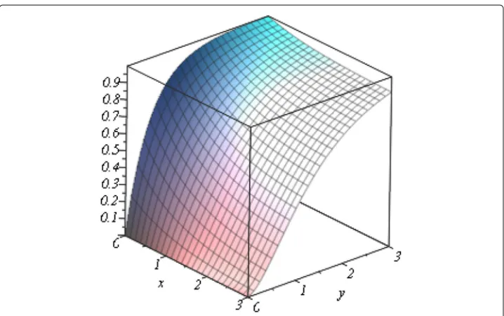
For investigating the proposed direct nonparametric quantile regression estimator in(7), in this Section, Monte Carlo simulations are performed. We generatem random sam-ples with sizeneach from the second kind of Gumbel’s bivariate exponential distribution Gumbel (1960) which has a non-linear conditional quantile function ofygivenxin(11). It has c.d.f.F(x,y)and density functionf(x,y)in(10):
F(x,y)=(1−e−x)(1−e−y)(1+αe−(x+y)), x≥0, y≥0, α >0, (10)
f(x,y)=e−(x+y)(1+α(2e−x−1)(2e−y−1)), x≥0, y≥0, α >0.
The conditional density ofyfor givenxis
f(y|x)=e−y(1+α(2e−x−1)(2e−y−1)), x≥0, y≥0, α >0.
The conditional c.d.f. ofyfor givenxis
F(y|x)=e−y(α(2e−x−1)(1−e−y)−1)+1, x≥0, y≥0, α >0.
The trueτth conditional quantile function ofygivenxof (10)is
ξ(τ|x)=Qy(τ|x)=ln
2α(2e−x−1)
α(2e−x−1)−1+(α(2e−x−1)+1)2−4ατ(2e−x−1)
, (11)
x≥0, α >0, 0< τ <1.
Lettingα=1, the c.d.f. in(10)is in Fig.1. We use three quantile regression methods:
1. The regular quantile regressionQR(τ|x)estimation based on(3):
QR(τ|x)=β0(τ) +β1(τ) x. 0< τ <1 (12)
2. The first-order linear polynomials Quantile Regression (LPQR)QLP(τ|x) (Chaud-huri1991, Keoker2005, Yu and Jones1998), forzin a neighborhood ofx,
QLP(τ|x)=a0(τ,x)+a1(τ,x)(z−x). 0< τ <1, (13)
Fig. 1The c.d.f. of Gumbel’s Second kind of bivariate exponential distribution withα=1
a(τ,x)=arg min β(τ)∈Rp
n
i=1
ρτ(yi−a0(τ,x)−a1(τ,x)(xi−x))K
x−xi h
, 0< τ <1,
herea(τ,x) = (a0(τ,x),a1(τ,x))T,handK are the bandwidth and kernel function. the LPQR can be computed by theRpackage ‘quantreg’ Koenker (2018).
3. The direct nonparametric quantile regressionQD(τ|x)estimation based on(7)
QD(τ|x)= n
i=1
Whx(x,Xi)ξi(τ|xi), 0< τ <1, (14)
whereξi(τ|xi)is obtained by(6), Whx(x,Xi)is given by(7).
For each method, we generate sizen=100,m=100 samples.QR,i(τ|x),QLP,i(τ|x)and QD,i(τ|x), i = 1, 2,. . .,m, are estimated in theith sample. Letα = 1 in(11).Then the trueτth conditional quantile is
ξ(τ|x)=Qy(τ|x)=ln
2e−x−1
e−x−1+e−2x−τ(2e−x−1)
, x≥0, α >0, 0< τ <1.
(15)
The simulation mean squared errors (SMSEs) of the estimators(12),(13)and(14)are:
SMSE(QR(τ|x)) = 1 m
m
i=1
N
0 (
QR,i(τ|x)−Qy(τ|x))2dx; (16)
SMSE(QLP(τ|x)) = 1 m
m
i=1
N
0 (
QLP,i(τ|x)−Qy(τ|x))2dx, (17)
SMSE(QD(τ|x)) = 1 m
m
i=1
N
0 (
QD,i(τ|x)−Qy(τ|x))2dx, (18)
Table 1Simulation Mean Square Errors (SMSEs) and Efficiencies (SEFFs) of Estimating
Qy(τ|x),m=100,n=100,N=6.
τ 0.95 0.96 0.97 0.98 0.99
SMSE(QR(τ|x)) 22.091 26.632 28.982 42.725 73.340
SMSE(QLP(τ|x)) 8.160 9.667 11.074 15.080 23.734
SMSE(QD(τ|x)) 5.161 6.630 6.552 8.850 11.596
Efficiency
SEFF(QLP(τ|x)) 2.7072 2.7449 2.6171 2.8332 3.0901
SEFF(QD(τ|x)) 4.2804 4.0169 4.4234 4.8278 6.3246
SEFF(QLP(τ|x))=
SMSE(QR(τ|x))
SMSE(QLP(τ|x)), SEFF(QD(τ|x))=
SMSE(QR(τ|x)) SMSE(QD(τ|x)),
whereSMSE(QR(τ|x)),SMSE(QLP(τ|x))andSMSE(QD(τ|x))are defined in(16), (17)and (18),respectively.
Table1shows that all of theSEFF(QD(τ|x))are larger than 1 whenτ =0.95,. . . , 0.99. Figure2compares theSMSE(QR(τ|x)),SMSE(QLP(τ|x))with theSMSE(QD(τ|x))for τ =0.95,. . ., 0.99. It demonstrates that allSMSE(QD(τ|x))have smaller values than both SMSE(QLP(τ|x))andSMSE(QR(τ|x)), thus, the simulation results show that the proposed estimatorQD(τ|x)is more efficient relative to the regular linear estimatorQR(τ|x)and nonparametric local polynomial estimatorQD(τ|x).
Next, we compareQD(τ|x)andQR(τ|x)in Figs.3and4.
Figure3shows the boxplots ofQR(τ|x)andQD(τ|x)forτ = 0.95, 0.97, and 0.99.(The true conditional quantiles are in blue line). TheQD(τ|x)has much smaller variance than QR(τ|x)s.
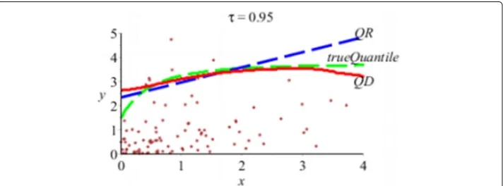
Figure4shows the average curves of the 100 estimatedτ = 0.95th quantile curves of QR(τ|x)(in blue dash line) and that ofQD(τ|x)(in red solid). The averageQD(τ|x)curve is much closer thanQR(τ|x)to the true quantile curve (in green dash).
Fig. 3Box plots for (a)τ=0.95th quantile curves; (b)τ=0.97th quantile curves; (c)τ=0.99th quantile curves. The true conditional quantile lines are in blue
From the overall results of the simulation, we can conclude that Table1and Figs.2,3, and4show that forτ = 0.95,. . ., 0.99, the proposed direct estimatorQD(τ|x) in(7)is more efficient relative to the regular regressionQR(τ|x)in(2)and a nonparametric LPQR in(13).
5 Real examples of applications
In this section, we apply the following two regression models to the Buffalo snowfall and CO2emission examples in Huang and Nguyen (2017):
1. The regular quantile regressionQR(τ|x)in model (2)using estimatorβ(τ) in(3); 2. The direct nonparametric quantile regressionQD(τ|x)in(7).
5.1 Buffalo snowfall example
Huang and Nguyen (2017) used the following linear second order polynomial quantile regression model for this example (National Weather Service Forecast Office2017):
Qy(τ|x)=β0(τ)+β1(τ)x+β2(τ)x2,
Table 2Buffalo Daily Snowfalls (cm) at High Quantiles UsingQRandQD
τ=0.97 τ=0.99
Temperature(◦C) QR QD QR QD
-15 37.38 25.49 105.46 60.64
-10 33.19 30.23 87.95 62.98
-5 30.98 33.33 72.08 56.54
0 30.73 29.89 57.86 54.56
5 32.47 33.27 45.29 52.39
10 36.17 37.34 34.36 43.04
whereyrepresents the total snowfall(cm)andxrepresents the maximum temperature
(◦C).
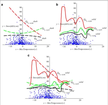
In this paper we use the proposed five-step algorithm in Section2to obtain the new direct nonparametric quantile estimatorQD(τ|x)in(7).We compare the new estimator QD(τ|x)with the regular quantile estimatorQR(τ|x)in Huang and Nguyen (2017). Table2 and Fig.5show the difference of values of two estimators. Figure5a,bandcshow the scatter plot of the daily snowfall vs. maximum temperature with the fittedQR, andQD
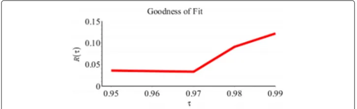
Fig. 6RelativeRτofQDrelative toQRfor the Buffalo snowfall example
quantile curves atτ =0,95, 0.97 and 0.99. It is interesting to see that theQDcurves appear to follow the data patterns closer than theQRcurves.
Table2lists the estimated Buffalo snowfall quantile values at a given maximum tem-perature forτ =0.97 and 0.99. It demonstrates that when quantiles are at highτ, theQD gives greater variety of snowfall predictions than theQR. The relationship of snowfall and max-temperature is not necessarily linear.
Figure 6 and Table 3 show the values of the Relative R(τ) in (9) for given τ = 0.95,. . ., 0.99. We note thatR(τ) >0 which means thatVD(τ) <VR(τ)andQDis a better fit to the data thanQR.
Figure5cshows that the proposed direct nonparametric quantile regressionQD pre-dicts that for moderate temperatures, such as 5◦C to 10◦C, it is likely to have smaller but varied snowfalls in Buffalo than the regular QD predicts. For temperature over 10◦C, the QD predicts a much higher value snow amount than the regular QR pre-dicts. On another side, for very low temperatures, such as −15◦C to 0◦C, the QD and QR both predict more likely to have extreme heavy snowfalls that may cause damage. Thus prediction of heavy snowfalls is related to cold weather forecasts. But the prediction snowfalls related to temperature from the QD is not as a simple lin-ear relationship as QR predicts. We also note that lots of snow occurred between -5◦C to 0◦C; the predictions form the QD are reflecting this fact and give varied predictions.
5.2 CO2emission example
Huang and Nguyen (2017) used the linear quantile regression model for this example:
Qy(τ|x1,x2)=β0(τ)+β1(τ)x1+β2(τ)x2,
where y represents CO2emission (tonnes) per capita,x1represents ln of gross domestic
product (GPD) (US $), per capita andx2represents ln of electricity consumption (E.C.)
(kilowatts) per capita (Carbon Dioxide Information Analysis Centre (2017)).
Similar as in the Buffalo Snowfall example in Subsection5.1, we use the proposed five-step algorithm in Section2to obtain the new direct nonparametric quantile estimator
Table 3RelativeR(τ)Values for the Buffalo Snowfall Example
τ=0.95 τ=0.96 τ=0.97 τ=0.98 τ=0.99
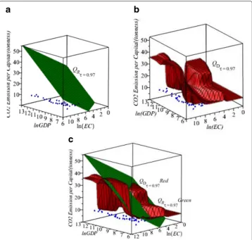
Fig. 73D Plots for CO2Emission, data−blue,n=123, (a) RegularQR−green atτ=0.97; (b) DirectQD− red atτ=0.97; (c) RegularQR−green and DirectQD−red in a plot atτ=0.97
Fig. 82D plots for CO2Emission, data−blue,n=123, (a) RegularQR(in dash) and directQD(in solid) of the CO2emission vs ln(GDP) when the country’s E.C. is 2980.96 kilowatts atτ=0.97 (green) and 0.99 (red). (b)
RegularQR(in dash) and directQD(in solid) of the CO2emission vs ln(E.C.) when the country’s GDP is
Table 4CO2Emission per capita at high quantiles given ln(GDP) estimatorsQRandQD
τ=0.97
ln of GDP per capita ($) QR QD
7.5 15.2181 8.8737
8 18.0437 10.1949
8.5 20.8693 11.7828
9 23.6950 14.4143
9.5 26.5206 19.0458
10 29.3462 24.0338
10.5 32.1718 27.9596
11 34.9975 31.1097
11.5 37.8231 30.7696
12 40.6487 31.2366
2980.96 Kilowatts of Electricity Consumed per capita
QD(τ|x)in(7).We compare the new estimatorQD(τ|x)with the regular quantile estima-torQR(τ|x)in Huang and Nguyen (2017). Figures7,8and Tables4,5show the differences of the values of two estimators. Figure7ashows the 3D scatter plot of CO2emission vs
ln(GDP) and ln(EC) with the fitted regularQRsurface atτ =0.97. Figure7bshows the 3D scatter plot of CO2emission vs ln(GDP) and ln(EC) with the fitted directQDsurface at τ =0.97. Figure7cshows the 3D scatter plot with both the regularQR(green) and direct QD(red) quantile surfaces of CO2emission vs the ln(GDP) and ln(E.C.) atτ =0.97. It is
interesting to see the difference between theQRandQDquantile surfaces.
We may see theQRandQDquantile curves more cleanly in 2D plots. Figure8ashows the 2D scatter plot of CO2emission vs ln(GDP) when the country’s E.C. is 2980.96
kilo-watts with the fitted regularQRand directQDcurves at at τ = 0.97. Figure8bshows the 2D scatter plot of CO2 emission vs ln(E.C.) when the country’s GDP is $13,359.73
with the fitted regularQR and directQD curves at atτ = 0.97. We note that the QR and QD quantile regression curves appear to fit the data. In general, the QD curves follow the data patterns closer than QR quantile lines, and theQD produces different estimated CO2emissions than theQRestimated at high quantiles. In Fig. 7, it is
inter-esting to see that theQDconditional quantile surfaces are not linear as the linear planes of theQR.
Tables4 and5provide details of the estimated high quantiles about countries’ CO2
emission atτ = 0.97 when the countries consume 2980.96 kilowatts of electricity and have a GDP of $13,359.73, respectively.
Table 5CO2emission per capita at high quantiles given ln(E.C.) estimatorsQRandQD
ln of Electricity Consumption τ=0.97
per capita (kilowatts) QR QD
0 6.9775 7.1919
2 11.8632 7.2759
4 16.7490 24.6924
6 21.6348 9.5560
8 26.5206 15.9569
10 31.4064 31.5634
12 36.2921 39.6481
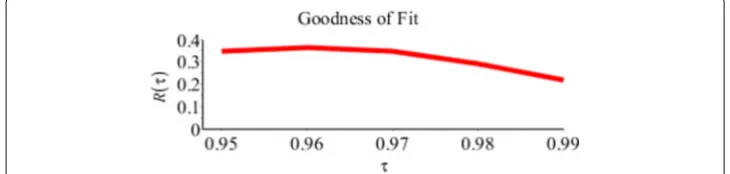
Fig. 9RelativeR(τ)ofQDrelative toQRfor the CO2emission example
Figure9and Table6show the RelativeR(τ)in(9),forτ = 0.95,. . ., 0.99. All values of RelativeR(τ)are larger than 0, which signifies thatVD(τ) < VR(τ)and it also suggests that the direct quantile regression estimatorQDis a better fit to the CO2emission data
than the regular quantile regression estimatorQR.
Over all, it is interesting to see that the proposed direct estimatorQDgave more vari-ety of predictions than theQRon CO2emissions relative to gross domestic product and
amounts of electricity produced. The relationships are not necessarily linear and model free. We expect that the predictions fromQDmay be more reasonable. The predictions may benefit prevention of further damages of CO2emissions to the environment.
6 Conclusions
After the above studies, we can conclude:
1. This paper proposes a new direct nonparametric quantile regression method which is model free. It uses nonparametric density estimation and nonparametric regression techniques to estimate high conditional quantiles. The paper provides a computational five-step algorithm which overcomes the limitations of the estimation in the linear quantile regression model and some other nonparametric quantile regression methods.
2. The Monte Carlo simulation works on the second kind of Gumbel’s bivariate expo-nential distribution which has a nonlinear conditional quantile function. The simulation is different from the bivariate Pareto distribution which has a linear conditional quantile function, in Huang and Nguyen (2017). The simulation results confirm that the proposed new method is more efficient relative to the regular quantile regression estimators and a local polynomial nonparametric estimator.
3. The proposed new direct nonparametric quantile regression can be used to predict extreme values of snowfall and CO2emission examples in Huang and Nguyen (2017). The
proposed direct quantile regressionQDestimator gives a variety of predictions which fits data very well. The prediction of relationships are not simply just linear. We expect that the predictions fromQDmay be more reasonable than the regular quantile regression predictions. The new estimator may benefit prevention of further damages of the extreme events to human and the environment.
4. The proposed direct nonparametric quantile regression provides an alternative way for quantile regression. Further studies on the details of this method are suggested.
Table 6RelativeR(τ)values for CO2emission example
τ=0.95 τ=0.96 τ=0.97 τ=0.98 τ=0.99
Acknowledgements
We are grateful for the comments of the reviewers and editor. They have helped us to improve the paper. This research is supported bythe Natural Science and Engineering Research Council of Canada(NSERC)grant MLH, RGPIN-2014-04621.We deeply appreciate the work and suggestions of Ramona Rat and Jenny Tieu which helped to improve the paper.
Authors’ contributions
The authors MLH and CN carried out this work and drafted the manuscript together. Both authors read and approved the final manuscript.
Competing interests
The authors declare that they have no competing interests.
Publisher’s Note
Springer Nature remains neutral with regard to jurisdictional claims in published maps and institutional affiliations.
Author details
1Department of Mathematics & Statistics, Brock University, St. Catharines, Ontario L2S 3A1, Canada.2Apotex Inc., Toronto,
Ontario M9L 1T9, Canada.
Received: 12 September 2017 Accepted: 31 May 2018
References
Carbon Dioxide Information Analysis Center (2017).http://www.cdiac.ornl.gov. Accessed 20 Oct 2014
Cai, Z: Applied Nonparametric Econometrics. Wang Yanan Institute for Studies in Economics, Xiamen University, China (2013)
Chaudhuri, P: Nonparametric estimates of regression quantile and their local Bahadur representation. Ann. Stat.2, 760–777 (1991)
Fukunaga, K: Introduction to Statistical Pattern Recognition. Academic press, New York (1972) Gumbel, EJ: Bivariate exponential distributions. J. Am. Stat. Assoc.55, 698–707 (1960)
Hall, P, Wolff, RCL, Yao, Q: Methods for estimating a conditional distribution. J. Am. Stat. Assoc.94, 154–163 (1999) Huang, ML, Nguyen, C: High quantile regression for extreme events. J. Stat. Distrib. Appl.4(4), 1–20 (2017)
Huang, ML, Xu, X, Tashnev, D: A weighted linear quantile regression. J. Stat. Comput. Simul.85(13), 2596–2618 (2015) Koenker, R: Quantile regression. Cambridge University Press, New York (2005)
Koenker, R. Package ‘guantreg’: Quantile Regression (2018). R Package, Version 5.35 (Available from https://www.r-project.org). Accessed 23 Apr 2018
Koenker, R, Bassett, GW: Regression Quantiles. Econometrica.46, 33–50 (1978)
Koenker, R, Machado, JAF: Goodness of fit and related inference processes for quantile regression. J. Am. Stat. Assoc. 96(454), 1296–1311 (1999)
Li, Q, Racine, JS: Nonparametric Econometrics-Theory and Practice. Prinston University Press, Oxford (2007) National Weather Service Forecast Office (2017).www.weather.gov/buf. Accessed 22 Sept 2014
Scott, DW: Multivariate Density Estimation, Theory, Practice and Visualization, second edition. John Wiley & Sons, New York (2015)
Silverman, BW: Density estimation for statistics and data analysis. Chapman & Hall, London (1986)
Wang, HJ, Li, D: Estimation of extreme conditional quantile through power transformation. J. Am. Stat. Assoc.108(503), 1062–1074 (2013)