ORIGINAL ARTICLE
Pierre Berard · Ping Yang · Hidefumi Yamauchi Kenji Umemura · Shuichi Kawai
Modeling of a cylindrical laminated veneer lumber I: mechanical properties
of hinoki (Chamaecyparis obtusa) and the reliability of a nonlinear fi nite
elements model of a four-point bending test
Abstract The weak point of cylindrical laminated veneer
lumber (LVL) when its structure, used as a column in build-ings, is submitted to compressive or fl exural loads is the butt joint. To improve the understanding of the behavior of this complex structure, a fi nite elements analysis was used, which required linear and nonlinear mechanical properties to be input in the model. This article is the fi rst of a series of reports concerning the determination of such properties, in this case hinoki (Chamaecyparis obtusa), which has been chosen for the purpose of the study. We used various methods to establish the elastic coeffi cients, viscoelastic parameters in three orthotropic directions, and plastic behavior in a direction parallel to the grain. As there are few references about the mechanical properties of this species, even in the elastic domain, we had to use a statistical model based on density to discuss the results obtained in the elastic domain. Then a fi nite element method model of a standard four-point bending test was set up to verify that the nonlinear mechanical models used for computation give accurate results that match those of the experiments.
Key words Hinoki · Mechanical properties · Finite elements
method
P. Berard (*) · K. Umemura · S. Kawai
Research Institute for Sustainable Humanosphere, Kyoto University, Gokasho, Uji, Kyoto 611-0011, Japan
Tel. +81-774-38-3670; Fax +81-774-38-3678 e-mail: [email protected]
P. Yang
Department of Technology Education, Faculty of Education, Kumamoto University, Kumamoto 860-8555, Japan
H. Yamauchi
Institute of Wood Technology, Akita Prefectural University, Noshiro 016-0876, Japan
Parts of this article were presented in the form of posters at the Inter-national Symposium on Wood Science and Technologies, Yokohama, Japan (2005) and the 2nd international symposium on veneer process-ing and products, Vancouver, Canada (2005)
Introduction
Cylindrical laminated veneer lumber (LVL) is a biomimetic structural product composed of several layers of veneer wound along a steel mandrel in a parallel to the grain (L) direction, thus presenting an angle of alternately +10° or –10° from the axis of the column designed to act as a post, or a vertical structural member. This kind of column is his-torically appreciated in Japan, as it has an important place in the structures of traditional buildings and temples. Such large-diameter columns, which have been used for a long time, are built from the whole stem of a tree or comprise an assembly of several parts to make a large column.
To reproduce these large-diameter columns, Sasaki1
turned peeled veneers into the form of a tape and then wound this product along a steel mandrel. After gluing in alternate directions for a suffi cient amount of layers, the steel mandrel is removed; and the column is fi nished by applying a thin layer of high-quality peeled veneer. This product has been found to be a good way to use low-grade veneers to make a high value-added product,1
although the winding process leaves a gap between the layers’ borders. This gap is known as the butt joint and appears to be one of the weaknesses of this structure.
To improve the quality of the butt joint, we decided to use a fi nite elements model (FEM) which, to be accurate, requires that we determine not only the elastic properties of the constitutive material but also the time-dependent properties. The aim of part of our overall study was to determine the dimensions of these mechanical properties.
Many species can be used to produce this cylindrical LVL, but for the purpose of this study we chose hinoki (Chamaecyparis obtusa) for its known homogeneity, which is supposed to ease studying LVL. Regarding Young’s modulus (modulus of elasticity, or MOE) and strength in the L direction, some information is already available for this species. Ikeda et al.2
performed a study on hinoki populations, where they established the parallel to the grain dynamic MOE of the trees using a tapping method. The measured value was 10 GPa for the class at 20–70
bending tests. They found that the MOE ranged from 9650 to 12 730 MPa (bending) and from 10 670 to 11 640 MPa (tensile), depending on the location of their growth period. The strength ranged from 59 to 86 MPa (bending) and from 114.3 to 137.9 MPa (tensile) depending on the location of their growth period. Respectively, the mean density ranged from 390 to 460 kg/m3
(bending) and from 390 to 450 kg/m3
(tensile). Ishimaru et al.4
proposed some results about the evolution of the transverse MOE [radial (R) direction] and strength of hinoki samples in regard to bending: 1005 MPa and 16 MPa, respectively, at 12% mois-ture content (MC).
Regarding time-dependent behavior, it is diffi cult to fi nd publications directly related to hinoki. However, Ishimaru et al.5
showed the relative relaxation modulus after a step bending strain during adsorption and desorption. They showed that the relative transverse modulus (R) is 86% during adsorption (at 33.1% MC) after 20 min of relax-ation) and 85% during desorption (at 22.8% MC after 20 min of relaxation).
To achieve our goal, we also had to perform some tests. As we had to determine the orthotropic elastic stiffness matrix of hinoki, instead of applying the standards (which would not have been time-effective) we decided to apply the single cube method.6
This is a fast, cost-effective way to determine the six elastic Young’s moduli and the Poisson ratios. The principle is to perform compression tests on cubic samples of 50 × 50 × 50 mm, each sample being tested several times in different directions to take into account the effects of variability. The stress range is supposed to let the samples be in their elastic domain, thereby allowing tests in the three main directions on the same sample. Because of the cubic geometry of the samples, it is easy to measure strains in parallel and transverse to the load direction. However, each test should retrieve the parallel and perpen-dicular to the load direction strain, allowing one to deter-mine Young’s modulus (by plotting the stress–strain curves) and the Poisson ratio in the three main directions. Owing to the diffi culty of measuring the small deformations perpen-dicular to the loading direction when loading in the R and T directions,7
we were not able to determine the RL/TL Poisson ratio. Instead, we used the value provided by the model of Guitard.8
This model, based on a determination of the elastic mechanical properties of various softwoods and hardwoods (density ranging from 260 to 590 kg/m3
in the case of the softwoods), provides the complete orthotropic elastic stiffness matrix based on the density and the mois-ture content.
To study viscoelastic behavior, we performed relaxation tests, applying a step strain to establish the relaxation moduli in the three natural directions. Regarding plastic behavior, we used compression tests to estimate the evolu-tion of the plastic strain as a funcevolu-tion of time, assuming that the total amount of strain measured was equal to the sum of the elastic strain, viscoelastic strain, and plastic strain.
test provides with those from experimental data gained from raw hinoki according to the French standard refer-enced as NF-EN-408.9
Materials and methods
Raw material
The raw material used for experiments consists in three trees of hinoki, grown in the Yoshino area, Nara Prefecture, Japan. They were 80–100 years old at the time of harvesting, with a diameter of around 30 cm at breast height. After harvesting, three logs of 1.3 m were cut in each tree from the bottom. Six of these nine logs (L1– L6) were stored in water to keep them saturated for the prospective peeling. The three remaining logs (L7– L9) were stored outside to be cut in samples for experiments.
Young’s modulus and Poisson ratio of raw hinoki: single cube method
The single cube method6
has been applied to determine Young’s modulus and the Poisson ratio of hinoki. This is a fast, effi cient way to determine these properties using a few cubic samples. Ten cubes (50 × 50 × 50 mm) were cut in clear, knot-free bark of hinoki from one of the L1 logs, their edges being aligned with the three natural directions. The samples were then stored in a conditioning room at 20°C and 65% relative humidity (RH) for 1 month to temper them at 12% moisture content (MC). Their exact dimen-sions were then measured using a digital caliper and weight, and their MC was established at 11.29%.
The tests consist in three successive compression tests performed on a 4411 Instron (Norwood, MA, USA) univer-sal testing machine equipped with a 5-kN load cell. The deformations were measured using a particle image velo-cimetry method,10
which was developed for fl ow motion analysis but can be applied to displacement fi eld measure-ments. The central area of each face was painted with a thin random speckling of black dots after applying a white uniform background. The pictures have been treated with a toolbox developed by Sveen and Cowan,11
designed for MATLAB (MatWorks, Natick, MA, USA). The result con-sists in the displacement fi eld of the concerned surfaces, which allows determining the deformations in and perpen-dicular to the testing direction. In each testing direction, we made sure to remain far under the elastic limit. To do so, preliminary tests were performed on an Instron model 1125 equipped with a 50-kN load cell to determine the Fmax values
Four-point bending Young’s modulus of raw hinoki: variation along the radius
Owing to the limitations of the load cell of the 4411 Instron machine, the parallel to the grain MOE could not be deter-mined using the single cube method. Therefore, we performed four-point bending tests on clear samples – dimensions: 20 mm (R) × 20 mm (T) × 400 mm (L) – according to the parameters of the French NF-EN-408 standard; and we took this opportunity to check the varia-tion in MOE along the radius. To do so, we cut 29 samples in different areas along the radius of the stem (Fig. 1), 7 located in the heart (H) area, 7 in the middle (M) area, 8 in the outer (O) area, and 7 in the sapwood (S) area. To reduce the indentation under the loading points, we used four steel plates (20 × 10 × 5 mm), as recommended in the NF-EN-408 standard, inserted between the sample and the fi xed and moving heads (Fig. 2).
Elastic shear modulus of raw hinoki
We applied the off-axis tensile test method as described by Xavier et al.12
This method requires the use of oblique end tabs (Fig. 3) that homogenize shear stress in the central area of the sample. We then used a two-dimensional FEM to determine, for each principal direction, the angle that mini-mized lateral displacement of the off-axis sample submitted to the tensile test. Based on this analysis, the end tabs angles (α) should be set at 55° (direction LR), 65° (LT), and 35° (RT). These results are similar with those of Xavier et al., who used a 55° end tabs angle for the LR direction.
The deformations were measured using strain gauges (KFG-8-120-D17-11; Kyowa Electronic Instruments, Tokyo, Japan) in the LT and LR planes and digital image correla-tion (same method and preparacorrela-tion of the samples as for Young’s modulus) in the RT plane, as the strain gauge cement was found to infl uence strongly the results in this direction by spreading in the wood structure. The strain gauges were welded to wires connected to a data logger that was connected to a computer. The testing machine was the 4411 Instron machine equipped with a 5-kN load cell.
Compression strength
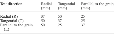
For compression strength, three series of 50 × 25 × 37 mm samples (Table 1) from the same bark were cut in the three natural directions, the direction of the load being along the 37-mm edge. These samples were been stored in a condi-tioning room at 20°C and 65% RH for 1 month; they were then weighed to determine their MC, which was 11.35%.
Testing was done with the Instron model 1125 machine equipped with a 50-kN load cell. To measure displacement of the crosshead, two linear displacement transducers (CP 25; Tokyo Sokki Kenkyujo, Tokyo, Japan) were fi xed on each side of the sample and were maintained on the fi xed part of the compression plate by magnetic arms. The moving heads of the transducers touched the moving part of the compression plate. The information from the transducers was collected through a data logger that was connected to a computer.
Shear strength
Shear strength was established using the JIS Z2101 standard method.13
The apparatus used for that purpose was the stan-dard in use in the laboratory for this test. As for the com-pression tests, testing was done with the Instron model 1125 machine equipped with a 50-kN load cell. To measure
Fig. 1. Positioning of the four-point bending samples
Fig. 2. Finite element method (FEM) model of a four-point bending test
Fig. 3. Off-axis tensile test sample. R, radial direction; T, tangential direction; L, parallel to the grain direction
Table 1. Orientation of the compression and relaxation test samples
Test direction Radial (mm)
Tangential (mm)
Parallel to the grain (mm)
Radial (R) 37 50 25
Tangential (T) 50 37 25
Parallel to the grain (L)
of the compression plate by magnetic arms. The moving heads of the transducers touched the moving part of the upper plate. The information from the transducers were collected through a data logger that was connected to a computer.
Tensile strength
The only values we found regarding tensile strength were in the article by Sano.3
Therefore, we decided to check whether there were correlations between density and the tensile strength in different softwoods in the existing litera-ture. The softwoods there were mainly American species, their properties being described in the Wood Handbook.14 Using the mean of those correlations, we defi ned a tensile strength that was equal in the R and T directions, as the
Handbook reported only the “perpendicular to the grain
tensile strength.”
Relaxation tests
To determine the time-dependent behavior of Young’s modulus, we performed relaxation tests on 50 × 25 × 37 mm samples (Table 1), the testing direction being aligned with the 37-mm edge. For those tests, we used the preprogrammed relaxation method that accompanied the 4411 Instron testing machine. We set the fi xed deformation at 10−3
for the R direction, 2 × 10⁻³ for the T direction, and 4 × 10⁻³ for the L direction. The strains were applied for 300 s. Then the variation in the load was measured directly from the load cell. After obtaining these points, the experimental data were fi tted using logarithm curves.
Plastic behavior
To estimate the plastic strain during bending, we used data from the compression tests performed on raw hinoki in the L direction. As the curves give the whole deformation, we used the results from relaxation tests (relaxation moduli) and the MOE in the L direction to isolate, by subtraction, the plastic strain. Then, the plastic strain for each sample was fi tted as a function of time and stress. Finally, we used the average of the determined coeffi cients of this function for the six tested samples. We also set the fi rst yield stress in accordance with the values from the bending tests per-formed on the raw material (i.e., 31 MPa).
Settings for the fi nite element model
An FEM of a four-point bending test applied to a 20 mm (R) × 20 mm (T) × 400 mm (L) sample was defi ned. Regard-ing the mechanical properties, the model was fed with the properties established during tests described previously. We used the properties of symmetry to reduce the size of the
plates (20 × 10 × 5 mm) under the loading and fi xed heads of the bending bench (to prevent indentation, exactly as it is done during the real tests). A contact analysis was run at each step, allowing the plates to slide under the fi xed or moving head (friction coeffi cient for steel/steel was 0.1). The steel plates were glued to the sample only on the extremities submitted to loading and the center for the one lying on the fi xed head; this step was taken to prevent wide movements of these plates at the fi rst step of the analysis, which would lead to failure. These settings prevent the plate to come reinforce the structure of the sample.
The criterion using for determining the equivalent fi rst yield point is the generalized plasticity criterion, which mainly requires fi rst yield stress. We also applied the built-in failure criteria of Tsai-Wu, Hoffman, and maximum stress15
using the strength values obtained in the experiments and the literature (tensile strength).
After successful computation, the force and displace-ment of the nodes submitted to load are shown to deter-mine the MOE according to:
E
I L
F F
d d
L
Z
= × × × −
− ⎛
⎝⎜ ⎞⎠⎟
5 324
1 2 1
2 1
IZ= ×b h 3
12
where IZ is the quadratic moment in Z direction; b is the
width of the sample (X direction); h is the height of the sample (Y direction); L is the span of the four-point bending bench, which here is 360 mm. F1= 0.1 × Fmax or the closest
value available, a function of the number of computing increments. F2= 0.4 × Fmax or the closest value available, a
function of the number of computing increments. d1 is the
displacement at the loaded node under the force F1 or the
force corresponding to the closest value available, a func-tion of the number of computing increments. d2 is the
dis-placement at the loaded node under the force F2 or the
force corresponding to the closest value available, a func-tion of the number of computing increments.
Results and discussion
Variations in the density and four-point bending modulus along the radius
Table 2 shows the variation in the density and MOE in the four locations determined along the radius. Let us compare the results to those of Sano3
for the same range of density: He reported 11.67 GPa to 12.61 GPa (specimens coming Koya, Kochi prefecture) for a mean density of 440 kg/m3
, whereas we found 11.72 GPa for a mean density of 446 kg/ m3
Table 2. Variations in density, MOE, and MOR during bending along the radius of a hinoki trunk
Trunk area Density (kg/m3)
MOE (GPa)
MOR (MPa)
Sapwood area (S) 418 (3.88%) 11.2 (4.00%) 65.74 (4.10%) Outer area (O) 439 (2.04%) 11.74 (6.38%) 69.51 (3.38%) Middle area (M) 450 (0.85%) 11.88 (7.87%) 71.02 (4.51%) Inner area (I) 475 (1.58%) 12.06 (7.42%) 74.21 (5.24%) Average 446 (5.36%) 11.72 (3.10%) 70.12 (14.91%)
Numbers in parentheses are the standard deviation (%) MOE, modulus of elasticity
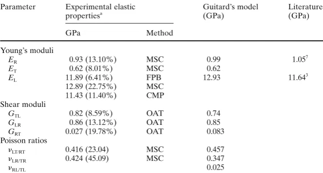
Table 3. Elastic properties measured with the single cube method and Guitard’s model
Parameter Experimental elastic propertiesa
Guitard’s model (GPa)
Literature (GPa)
GPa Method
Young’s moduli
ER 0.93 (13.10%) MSC 0.99 1.05
7
ET 0.62 (8.01%) MSC 0.62
EL 11.89 (6.41%) FPB 12.93 11.64
3
12.89 (22.75%) MSC 11.43 (11.40%) CMP Shear moduli
GTL 0.82 (8.59%) OAT 0.74
GLR 0.86 (13.12%) OAT 0.85
GRT 0.027 (19.78%) OAT 0.083
Poisson ratios
LT/RT 0.416 (23.04) MSC 0.457
LR/TR 0.424 (45.09) MSC 0.347
RL/TL 0.025
Numbers in parentheses are the standard deviation (%)
MSC, method of the single cube; FPB, four-point bending; CMP, compression; OAT, off-axis tensile
along the radius is about 5.36% and the variation in the MOE about 3.10%, confi rming the homogeneity of this wood.
The modulus of rupture (MOR) in the four-point bending tests was 70.12 MPa (14.91%), which is a little lower than that in Sano’s report (78.40 MPa), with the fi rst yield point (measured at 0.2% permanent deformation) at 27.61 MPa (1.50%). The relation between MOE and MOR (MOR = 0.00827 × MOE – 26.64) shows a good correlation (R2 =
0.9998), as does the relation between density and MOE (MOE = 17.785 × 10⁻³×
density + 3.779) (R2=
0.989).
Elastic properties of raw hinoki: results
The values (Table 3) determined using the single cube method were found to match well with those we obtained from the literature related to hinoki. The highest standard deviation was measured with the single cube method in the L direction (12.89 MPa, 22.75% SD). The strains measured in this case were close to 0.5 × 10⁻⁴
and sometimes less than one pixel in displacement, which induces higher error.10
Moreover, the mean value in the L direction provided a density similar to that found using Guitard’s model (12.93 MPa).
The most important difference between Guitard’s model, on one hand, and the experimental results, on the other hand, lies in the shear moduli. If the GLR is really
compa-rable that of Guitard’s model, the GTL (11.50% higher with
Guitard’s model) and especially GRT (67.40% lower) look
quite different than what we could expect. However, it must be mentioned that in the case of the shear properties the regression factor (R) of Guitard’s model for GTL was 0.533,
0.46 for GRT, and 0.67 for GLR. The quality of the regressions
of these moduli can explain the difference between the experimental numbers and those obtained using Guitard’s model.
Regarding Poisson ratios obtained using the single cube method, despite their nonnegligible standard deviations they have been used because, as absolute values, they are not so different from what we would expect according to Guitard’s model (9.05% difference compared to the model for LT/RT and 22.21% for LT/RT).
Strength properties of raw hinoki
Table 4 displays the strengths obtained with compression tests and the Japanese Standard JIS Z210113
in the three natural directions of wood. The values obtained from the compression and Japanese Standard shear tests show good homogeneity, the highest standard deviation being 11.93% for the compression strength in the T direction. It must be noted that the shear strengths show good correlation (R2=
0.995) with the shear moduli, not depending on the direc-tion. The shear values were found to be comparable to the only value we found in the literature.
Time dependence of Young’s modulus properties of raw hinoki
After establishing the equation of the plastic strain as a function of time, we were able to determine the whole deformation as a function of the time using the relations described below and compare it with the experimental data. The calculated curves were found to match well, sample by sample. Practically, experimental and calculated curves cannot be distinguished.
We input the average plastic strain (average of the C2
and C3 coeffi cients) in the FEM model of the four-point
bending test. The fi rst yield stress was set based on the value determined during the bending test on raw hinoki in the form of a ratio between the fi rst yield stress during bending and the fi rst yield stress during compression, which are involved in expression of the plastic strain.
Four-point bending test FEM model
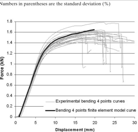
These data (elastic moduli, viscoelastic and plastic param-eters, strengths) were then input in the FEM of a four-point bending test and the computation was performed. Figure 4 shows the experimental four-point bending curves with, in addition, the force–displacement curve determined by the FEM. The fi nite elements curve has been artifi cially shifted to verify that it matches with the experimental one. One can visually note that the FEM curve falls right in the mean of the experimental data in both linear and nonlinear domains. The experimental data gave a MOE of 11.89 GPa, and we got 11.61 GPa from the FEM curve between the same
Table 5. Fitting relations of the viscoelastic behavior of raw hinoki
Fitting relation: σ (t) = C0× ln (t + 1) + (C1×σ0)
σV−R (t) =−3.84 × 10
−2× ln (t + 1) +σ
0 (C1= 1)
σV−T (t) =−3.707 × 10
−2× ln (t + 1) +σ
0 (C1= 1)
σV−L (t) =−4.029 × 10
−2× ln (t + 0.3) + (0.987 ×σ 0)
Direction Standard deviation of C0
Average of the regression coeffi cient (R2) of the fi tting
R 3.30% 0.938 (4.59%)
T 6.96% 0.954 (4.79%)
L 28.96% 0.879 (14.83%)
Numbers in parentheses are the standard deviation (%)
C2 0.0385 (28.30%)
C3 0.032 (26.90%)
Numbers in parentheses are the standard deviation (%) Compression
R 6.30 (8.57%)
T 6.70 (11.93%)
L 37.10 (3.59%)
Shear
LT 19.31 (3.09%)
LR 21.31 (2.67%)
RT 4.97 (5.93%)
Tensile strength
R 3.002
T 3.002
L 110.803
Numbers in parentheses are the standard deviation (%)
combination of the Maxwell or Kelvin-Voigt models. We simply pretended to get the raw data, fi t them to a function of time to be easily input in the FEM software. Thus, the curves display the evolution of the stress after a given defor-mation has been applied to the samples. The curves were then fi tted with equations as a function of time (Table 5).
For determining plastic strain, these relaxation tests were used as they caused a variation in MOE, the instant stress divided by the initial deformation giving an instant modulus
E(t) to determine the relaxation modulus. Considering the
fact that a four-point bending test lasts an average of 150 s, the viscoelastic effect causes a variation in the parallel to the grain MOE of about 3.8% during this kind of test. The variations are higher in the R and T directions (respectively, 16.05% and 16.5%). Ishimaru et al.5
reported a variation of about 12% after 5 min of desorption at 22.8% MC and 10% after 5 min of adsorption (at 33.1% MC); thus, our values were a little higher, considering that Ishimaru et al. had higher variations for higher moisture content.
Plasticity
We subtracted the elastic strain and the viscoelastic strain from the total experimental strain obtained with the com-pression test. The remaining strain, assumed to be the expression of plasticity, was fi tted using two coeffi cients (Table 6).
εplast= ×(σ L)× −
(
)
×
( )
C E eC t
1 0 1 2
values of F1 = 149 N and F2= 596 N, the difference being
2.35%.
In addition, the average experimental MOR was 71.12 MPa (SD 14.91%), and the average experimental dis-placement corresponding to the rupture was 17.81 mm (SD 25.50%). For the corresponding displacement, the FEM curve gave 74.51 MPa, which means 4.10% difference between the FEM analysis and the experimental data.
According to the failure criteria, rupture on the tensile side of the sample should occur at 70.22 MPa (Tsai-Wu), 63.74 MPa (Hoffman), or 65.63 MPa (maximum stress). The Tsai-Wu method shows 1.95% difference between the experimental and FEM results, with the Hoffman and maximum stress methods having greater differences (respectively, 11.00% and 8.43%).
Conclusion
The FEM analysis has been found to describe well the behavior of the material submitted to a four-point bending test in both linear and nonlinear domains. The experimental MOE was found to be only 2.35% different from that of the FEM analysis, and the FEM curve reached the same values (4.10% difference) of force at the displacement correspond-ing to rupture in the experiments.
Furthermore, the MOR determined using the Tsai-Wu, Hoffman, and maximum stress criteria were found to match very well with the experimental MOR obtained from bending tests. The Tsai-Wu criterion was particularly accu-rate, and the maximum stress criterion was farther from the experimental results (at 11.00%).
The FEM model as it is set up and the linear and non-linear mechanical properties applied can be considered reli-able for the purpose of describing the linear and nonlinear behaviors during four-point bending, including the predic-tion of rupture. These parameters can thus be applied to the study of complex LVLs, to see if we can obtain the same accuracy, as it would be interesting to be able to describe the behavior and estimate the rupture of these products.
For that purpose, we will apply these results and param-eters to studying the behavior of a cylindrical LVL, dis-cretized in the shape of a fl at part of a cylindrical wall.
Acknowledgments The authors thank the Japanese Society for the Promotion of Science, which has supported this study and the related work.
References
1. Sasaki H (1997) New technologies and machines for conversion of low-grade logs into value-added products. In: Proceedings of the fi rst international tropical conference, Kuala Lumpur, Malaysia, B-27
2. Ikeda K, Kanamori F, Arima T (2000) Quality evaluation of stand-ing trees by stress wave propagation method and its application. IV. Application to quality evaluation of hinoki (Chamaecyparis obtusa) forests. Mokuzai Gakkaishi 46:602–608
3. Sano E (1962) On the mechanical properties of Japanese hinoki-wood. Mokuzai Gakkaishi 8:7–12
4. Ishimaru Y, Arai K, Mizutani M, Oshima K, Iida I (2001) Physical and mechanical properties of wood after moisture conditioning. J Wood Sci 47:185–191
5. Ishimaru Y, Oshima K, Iida I (2001) Changes in the mechanical properties of wood during a period of moisture conditioning. J Wood Sci 47:254–261
6. Seichepine JL (1980) Mise au point d’une méthode expérimentale destinée à l’identifi cation de la matrice des complaisances élas-tiques des solides anisotropes: application au matériau bois. PhD thesis, I.N.P. de Lorraine
7. Gautherin MT (1980) Critère de contrainte limite du bois massif. PhD thesis, Université Pierre et Marie Curie, Paris, VI:113 8. Guitard D (1987) Mécanique du matériau bois et composites.
Cepadues Editions, Toulouse, France
9. Association Francaise de Normalisation (2004) NF-EN-408: struc-tural timber and glued laminated lumber. AFNOR, France 10. McKenna SP, McGillis WR (2002) Performance of digital image
velocimetry processing techniques. Experiments Fluids 32:106– 115
11. Sveen JK, Cowen EA (2004) Quantitative imaging techniques and their application to wavy fl ows. In: Grue J, Liu PL, Pedersen GK (eds). PIV and water waves. World Scientifi c, Singapore
12. Xavier JC, Garrido NM, Oliveira M, Morais JL, Camanho PP, Pierron F (2004) A comparison between the Iosipescu and off-axis shear test methods for the characterization of Pinus pinaster Ait. Composites Part A 35:827–840
13. Japanese Industrial Standard (2004) JIS Z2101: methods of test for wood
14. Forest Products Laboratory (1999) Wood handbook: wood as an engineering material. General technical report FPL:GTR-113. US Department of Agriculture, Forest Service, Madison, WI