R E S E A R C H
Open Access
Pipeline synthesis and optimization of
FPGA-based video processing applications with CAL
Ab Al-Hadi Ab Rahman
*, Anatoly Prihozhy and Marco Mattavelli
Abstract
This article describes a pipeline synthesis and optimization technique that increases data throughput of FPGA-based system using minimum pipeline resources. The technique is applied on CAL dataflow language, and designed based on relations, matrices, and graphs. First, the initial as-soon-as-possible (ASAP) and as-late-as-possible (ALAP) schedules, and the corresponding mobility of operators are generated. From this, operator coloring technique is used on conflict and nonconflict directed graphs using recursive functions and explicit stack
mechanisms. For each feasible number of pipeline stages, a pipeline schedule with minimum total register width is taken as an optimal coloring, which is then automatically transformed to a description in CAL. The generated pipelined CAL descriptions are finally synthesized to hardware description languages for FPGA implementation. Experimental results of three video processing applications demonstrate up to 3.9× higher throughput for pipelined compared to non-pipelined implementations, and average total pipeline register width reduction of up to 39.6 and 49.9% between the optimal, and ASAP and ALAP pipeline schedules, respectively.
1 Introduction
Data throughput is one of the most important para-meters in video processing systems. It is essentially a measure of how fast data passes from input to output of a system. With increasing demands for larger resolution images, faster frame rates, and more processing require-ments through advanced algorithms, it is becoming a major challenge to meet the ever-increasing desirable throughput.
For algorithms that can be performed in parallel, such as the case with most digital signal processing (DSP) applications, parallel platforms such as multi-core CPU, many-core GPU, and FPGA generally results in higher throughput compared to traditional single-core systems. Among these parallel platforms, FPGA systems allow the most parallel operations with the highest flexibility for programming parallel cores. However, register trans-fer level (RTL) designs for FPGA are known to be diffi-cult and time consuming, especially for complex algorithms [1]. As time-to-market window continues to shrink, a new high-level program that synthesizes to effi-cient parallel hardware is required to manage complex-ity and increase productivcomplex-ity.
The CAL dataflow language [2] was developed to address these issues, specifically with a goal to synthe-size high-level programs into efficient parallel hardware (see Section 3.2). CAL is an actor language in which program executes based on tokens; therefore, suitable for data intensive algorithms such as in DSP that oper-ates on multiple data. The language was also chosen by the ISO/IECaas a language for the description and spe-cification of videocodecs.
CAL design environment was initiated and developed by Xilinx Inc. and later became Eclipse IDE open source plugins calledOpenDF andOpenForge [3] which allow designers to simulate CAL models and synthesize to hardware description languages (HDL). The tools only perform basic optimizations for a given CAL actor for HDL synthesis; the final result highly depends on the design style and specification. Reference [4] presents coding recommendations for CAL designers to achieve best results. However, some optimizations are best per-formed automatically rather than manually, for example pipeline synthesis and optimization of CAL actors.
In CAL designs, actions execute in a single-clock cycle (with exception to while loops and memory access). Large actions, therefore, would result in a large combi-natorial logic and reduces the maximum allowable oper-ating frequency which in turn decreases throughput.
* Correspondence: [email protected]
SCI-STI-MM, Ecole Polytechnique Fédérale de Lausanne, 1015 Lausanne, Switzerland
The pipeline optimization strategy is to partition this large action into smaller actions that satisfy a required throughput requirement, but with a minimum resource penalty. Finding a pipeline schedule that minimizes resource is a nonlinear optimization problem, where the number of possible solutions increases exponentially with a linear increase of operator mobility.
This study presents an automatic non-pipelined CAL actor transformation to resource-optimal-pipelined CAL actors that meet a required stage-time constraint. The objective is to allow designers to rapidly design complex DSP hardware systems using CAL dataflow language, and use our tool to obtain higher throughput with opti-mized resources by pipelining the longest action in the design. In order to evaluate the efficiency of our metho-dology, three video processing algorithms are designed and used for pipeline synthesis and optimization.
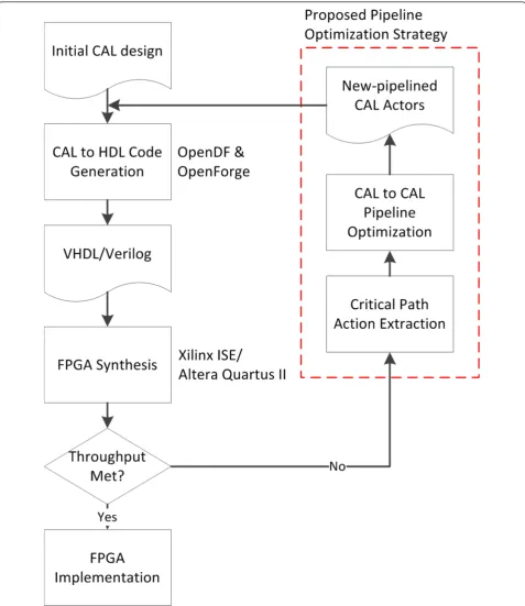
Figure 1 shows CAL to HDL design flow methodology with our CAL to CAL pipeline optimization strategy. Starting with an initial CAL design, it is first synthesized to HDL, then to a specific FPGA technology where the critical path and maximum allowable frequency infor-mation can be obtained. If the throughput requirement is met, the design can be implemented directly into the FPGA. In the case when a higher throughput is required, the action with the critical path is extracted from the design, and automatically pipelined with the required delay (for that actor) with minimum resource penalty. The original non-pipelined CAL actor is then replaced by the newly generated pipelined CAL actors. This process is repeated until the desired system throughput is achieved.
This article is organized as follows. The next section provides background and related study on pipeline synthesis and optimizations. Section 3 presents the basics of dataflow modeling in CAL. Following this, in Sections 4 and 5, we present our approach to pipeline synthesis and optimization using mathematical formula-tions. Then, in Section 6, experimental results are shown for several video processing applications, and finally, the last section concludes the article.
2 Pipeline synthesis and optimization: background
In computing, a pipeline is a set of data processing ments connected in series, so that the output of one ele-ment is the input of the next one. The eleele-ments of a pipeline are executed in parallel or in time-sliced fash-ion; in this case, some amount of buffer storage (pipe-line registers) is inserted in between elements. The time between each clock signal is set to be greater than the longest delay between pipeline stages, so that when the registers are clocked, the data that is written to the fol-lowing registers is the final result of the previous stage.
A pipelined system typically requires more resources (circuit elements, processing units, computer memory, etc.) than one that executes one batch at a time, because each pipeline stage cannot reuse the resources of the other stages.
Key pipeline parameters are number of pipeline stages, latency, clock cycle time, delay, turnaround time, and throughput. A pipeline synthesis problem can be con-strained either by resource or time, or a combination of both [5]. A resource-constraint pipeline synthesis limits the area of a chip or the available number of functional units of each type. In this case, the objective of the schedu-ler is to find a schedule with maximum performance, given available resources. On the other hand, a time-con-straint pipeline synthesis specifies the required throughput and turnaround time, with the objective of the scheduler is to find a schedule that consume minimum resources.
Sehwa [6] is the first pipeline synthesis program. For a given constraint on the number of resources, it imple-ments a pipelined datapath with minimum latency. Sehwa minimizes time delay using a modified list sche-duling algorithm with a resource allocation table. HAL [7] performs a time-constrained, functional pipelining scheduling using the force directed method which is modified in [8]. The loop winding method was proposed in the Elf [9] system. A loop iteration is partitioned hor-izontally into several pieces, which are then arranged in parallel to achieve a higher throughput. The percola-tion-based scheduling [10] deals with the loop winding by starting with an optimal schedule [11] which is obtained without considering resource constraints. Spaid [12] finds a maximally parallel pattern using a linear programming formulation. ATOMICS [13] performs loop optimization starting with estimating a latency and inter-iteration precedence. Operations which cannot be scheduled within the latency are folded to the next iteration, the latency is decreased, and the folding is applied again. The above-listed tools support resource sharing during pipeline optimization.
Pipelining is an effective method to optimize the execution of a loop with or without loop carried depen-dencies, especially for DSP [8]. Highly concurrent imple-mentations can be obtained by overlapping the
execution of consecutive iterations. Forward and back-ward scheduling is iteratively used to minimize the delay in order to have more silicon area for allocating addi-tional resources which in turn will increase throughput.
Another important concept in circuit pipelining is Retiming, which exploits the ability to move registers in the circuit in order to decrease the length of the longest path while preserving its functional behavior [15-17]. A sequential circuit is an interconnection of logic gates and memory elements which communicate with its environment through primary inputs and primary out-puts. The performance optimization problem of pipe-lined circuits is to maximize the clocking rate or equivalently minimize the cycle time of the circuit. The aim of constrained min-area retiming is to constrain the number of registers for a target clock period, under the assumption that all registers have the same area, the min-area retiming problem reduces to seeking a solution with the minimum number of registers in the circuit. In the retiming problem, the objective function and con-straints are linear, so linear programming techniques can be used to solve this problem. The basic version of retiming can be solved in polynomial time. The concept of retiming proposed by Leiserson et al. [15] was extended to peripheral retiming in [16] by introducing the concept of a “negative” register. These studies assume that the degree of functional pipelining has already been fixed and consider only the problem of adding pipeline buffers to improve performance of an asynchronous circuit.
The studies discussed are mainly targeted at the gen-eration and optimization of hardware resources from behavioral RTL descriptions. As to our knowledge, there is no available tool that performs these functions at the level of a dataflow program. The recent development of the CAL dataflow language allows the application of these techniques at a higher abstraction level, thus pro-vide the advantages of rapid design space exploration to explore pipeline throughput and area trade-off, and sim-pler transformation of a non-pipelined to a pipelined behavioral description, compared to low abstraction level RTL. The next section presents background on dataflow networks, high-level modeling for hardware synthesis, and the CAL actor language.
3 Dataflow modeling and high-level synthesis
Early studies on dataflow modeling are based on the Kahn process network introduced by Kahn in 1974 [18], which is a dataflow network with a local sequential pro-cess and global concurrent propro-cesses. This has been extended to graph models with a number of variants such as the directed acyclic graphs (DAG) [19-21] where each node represents an atomic operation, and edges represent data dependencies. The extension of the DAG is the synchronous dataflow graphs (SDF) [22] that annotates the number of tokens produced and con-sumed by the computation node, thus allowing feasible actor scheduling. Another type of dataflow graph is the
control dataflow graphs (CDFG) [23] which describes static control flow of a program using the concept of a director that regulates how actors in the designfireand how tokens are used.
Several dataflow implementation methodologies have been proposed to use pre-configured IP blocks in a data-flow environment such as the PICO framework [24], sim-pleScalar [23], and the study of Lahiri et al. [25]. There exist also commercial tools to aid DSP hardware designs such as Cadence SPW [26], Altera DSP Builder [27] and Xilinx AccelDSP [28]. Some of these offer integration with Mathworks MATLAB and SIMULINK [29]. These methods, however, constraint the design to a given class of architecture and put restrictions on designers.
In contrast to block-based DSP, C language, on the other hand, offers higher flexibility. Synthesis from C to hardware has been a topic of intensive research with developments such as the Spark framework [30], GAUT tool of LABSTICC [31], and Catapult C from Mentor Graphics [32]. However, C program is designed to exe-cute sequentially, and it still remains a difficult problem to generate efficient HDL codes from C, especially for DSP applications. Furthermore, C programs are also dif-ficult to analyze and identify for potential parallelism because of the lack of concurrency and the concept of time [33]. In the context of RTL, SystemC was intro-duced but mainly restricted to system level simulations and offered limited support for hardware synthesis. Transaction level modeling raises the abstraction level one step above systemC, and has gained popularity, but the level of abstraction remains quite low for effective designs.
High-level synthesis methodologies have also been used to generate pipeline schedules in RTL, for example in [34], where a variation of the Modulo scheduling algorithm has been used to exploit loop-parallelism by means of executing operations from consecutive itera-tions of a loop in parallel. The technique is applied on the level of an assembly language for generating pipe-lined RTL descriptions. However, besides the limitation of the technique on loop algorithms, the level of the input description is sequential and again, faces the ana-lyzability problem for effective pipelining. The study reported an improvement of up to 35% between pipe-lined and non-pipepipe-lined implementations.
In order to overcome these issues in the state of the art of high-level modeling and synthesis, the Ptolemy project at the University of California-Berkeley led to the development of the CAL dataflow language based on the concept ofactors.
3.1 Actor-based dataflow modeling
since then become widely used [1-4,36-41], especially in embedded systems, where actor-oriented design is a nat-ural match to the heterogeneous and concurrent nature of such systems.
Many embedded systems have significant parts that are best conceptualized as dataflow systems, in which actors execute and communicate by sending each other packets of data. It is often useful to abstract a system as a structure of cooperating actors. Many such systems are dataflow-oriented, i.e. they consist of components whose ability to perform computation depends on the availability of sufficient input data. Typical signal pro-cessing systems, and also many control systems fall into this category.
Component-based design is an approach to software and system engineering, in which new software designs are created by combining pre-existing software compo-nents. Actor-oriented modeling is an approach to sys-tems design, where entities called actors communicate with each other through ports and communication chan-nels. From the point of view of component-based design, actors are the components in actor-oriented modeling.
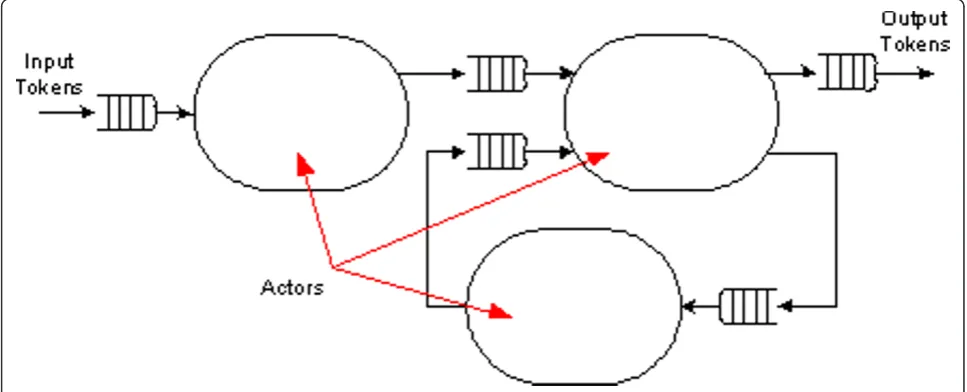
Figure 2 shows a simple dataflow network. Several actors are composed into a network, a graph-like struc-ture (often referred to as a model) in which output ports of actors are connected (typically with FIFO buf-fers) to input ports of the same or other actors, indicat-ing that tokens produced at those output ports are to be sent to the corresponding input ports. Such actor net-works are of course essential to the construction of complex systems. The encapsulation of each actor means that they are treated as a separate entity that works independently, but concurrently in a network. Increasing the number of actors in the network implies
more concurrent operations; which is analogous to pipelining.
3.2 CAL dataflow language
CAL is a domain-specific language for writing dataflow actors, with the final language specification released at the end of 2003 [36]. The language describes an algorithm using an encapsulated actor, which communicates with another actor by passing datatokens. An actor then per-forms its algorithm specified in itsactionif there is token available and if it is enabled by one or more of the follow-ing:guard, priority, andschedulingconditions. If an action is performed, it is said to befired, which consumes the input token, modify its internal states (variables, guard, schedule) and produces an output token which can be passed to another actor, itself or the system output [2]. An example of a CAL actor is given in Section 4.
CAL, however, is not a general purpose or full-fledged programming language; one of its key goals is to make actor programming easier by providing a concise high-level description with explicit dataflow keywords, unlike traditional programming languages. It is also designed to be platform independent and retargetable to a rich variety of target platforms, for example single-core and multi-core CPUs [1,36,41], FPGAs [1,37,39], and ASICs [38]. CAL provides a strict semantics for defining actor computa-tional operations, ports and parameters and its composite data structures. But it leaves certain issues to the embed-ding environment, such as the choice of supported data types and the definition of the target semantics.
3.3 CAL to HDL synthesis
The synthesis of CAL program to HDL is one of the core components of the CAL dataflow language. It was
pioneered by Xilinx Inc. and now available as Eclipse IDE opensource plugins called OpenDF and OpenForge [3]. The CAL to HDL code generator is essentially an XML processing and transformation engine using Java. The two main steps are:
1. Generation of top level VHDL from a flattened
CALdataflow network. The tool takes in a flattened CAL network called XDF, and transforms it into a top-level VHDL file. Some of the operations include port evaluation, data width, fanout, and buffer size annotation, and instance name addition.
2.Generation of Verilog files for eachCALactor. CAL actors are first checked syntactically, and then parsed into various XML representations that include several basic optimization steps. The final XML representation is called SLIM, which is a representation in a single-sta-tic assignment (SSAb) form. SLIM file is then loaded into a JavaDesignclass that represents top-level hard-ware implementation. The Java object representing the actor is optimized for hardware which includes opera-tor constant rule, loop unrolling, variable re-sizer, memory reducer, splitter and trimmer. Next, a hard-ware scheduler is also generated based on the specifica-tion in the SLIM representaspecifica-tion. Finally, a completed design object for an actor is written as a Verilog file.
HDL code generation from CAL actors has proven to generate efficient hardware. As reported in [37] for the hardware implementation of MPEG-4 Simple Profile Decoder, CAL design results in less coding, smaller implementation area, and higher throughput compared to classical RTL methodology.
The strength of the CAL dataflow language, especially for parallel DSP application, and its HDL synthesis makes it interesting for further optimization. As described, the CAL to HDL synthesis tool optimizes and generates code for each actor; no study has been done on actor partition-ing for pipelinpartition-ing, which is the focus of this article.
4 Mathematical modeling of pipeline synthesis and optimization
In order to clearly present our mathematical formula-tion of the pipeline synthesis and optimizaformula-tion, the theo-retical model will be complemented with a simple example–the YCrCb to RGB converter actor. A brief introduction to this actor will be given first.
4.1 The YCrCb to RGB conversion actor
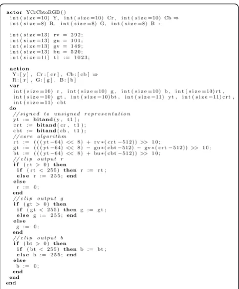
Figure 3 shows a CAL description of a 30-bit YCrCb to 24-bit RGB, based on Xilinx XAPP930 [42]. It is typi-cally used in high quality down-sampling and decoding of color spaces. The actor contains a single action that
first converts 10-bit inputs into an explicit 11-bit unsigned representation using thebitandoperation. Fol-lowing this, the core algorithm is performed using 11 adders/subtractors, 4 multipliers, and 6 shifters. Finally, the RGB output has to be clipped if the result exceeds the 8-bit per output dynamic range. This utilizes six if
statements with comparators.
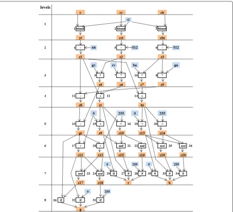
The general idea in our pipeline synthesis is to parti-tion this relatively large acparti-tion into several acparti-tions in separate actors. The first step is to make the action body (i.e. operations) more analyzable. This is achieved by limiting each arithmetic operator to two operands, and assigning a unique output variable for each opera-tor, essentially transforming each operator to a two-operands-single-assignment form. The dataflow graph of this transformation is given in Figure 4. Twenty extra variables (z1 toz20) are introduced to represent inter-mediate results of 35 operations.
The remainder of this section provides relations, graphs, and algorithms that define pipeline synthesis and optimization problem from a generic dataflow graph, with an example using the graph of Figure 4.
4.2 Dataflow graph relations
4.2.1 Operator precedence relation on dataflow graph LetN= {1, ...,n} be a set of algorithm operators andM= {1, ...,m} be a set of algorithm variables. The following
actor YCrCbtoRGB ( )
i n t ( s i z e =10) Y, i n t ( s i z e =10) Cr , i n t ( s i z e =10) Cb⇒
i n t ( s i z e =8) R, i n t ( s i z e =8) G, i n t ( s i z e =8) B : i n t ( s i z e =13) rv = 2 9 2 ;
i n t ( s i z e =13) gu = 1 0 1 ; i n t ( s i z e =13) gv = 1 4 9 ; i n t ( s i z e =13) bu = 5 2 0 ; i n t ( s i z e =11) t 1 := 1 0 2 3 ;
action
Y : [ y ] , Cr : [ c r ] , Cb : [ cb ]⇒
R : [ r ] , G : [ g ] , B : [ b ]
var
i n t ( s i z e =10) r , i n t ( s i z e =10) g , i n t ( s i z e =10) b , i n t ( s i z e =10) r t , i n t ( s i z e =10) gt , i n t ( s i z e =10) bt , i n t ( s i z e =11) yt , i n t ( s i z e =11) c r t , i n t ( s i z e =11) c b t
do
// s i g n e d t o u n s i g n e d r e p r e s e n t a t i o n
yt :=bitand( y , t 1 ) ; c r t := bitand( cr , t 1 ) ; c b t := bitand( cb , t 1 ) ;
// c o r e a l g o r i t h m
r t := ( ( ( yt−64)<<8 ) + rv∗( c r t−512))>>1 0 ;
g t := ( ( ( yt−64)<<8 )−gu∗( cbt−512)− gv∗( c r t−512))>> 1 0 ; bt := ( ( ( yt−64)<<8 ) + bu∗( cbt−512))>>1 0 ;
// c l i p o u t p u t r
i f ( r t> 0 ) then
i f ( r t< 2 5 5 ) then r := r t ;
e l s e r := 2 5 5 ;end e l s e
r := 0 ;
end
// c l i p o u t p u t g
i f ( g t> 0 ) then
i f ( g t< 2 5 5 ) then g := g t ;
e l s e g := 2 5 5 ; end e l s e
g := 0 ;
end
// c l i p o u t p u t b
i f ( bt> 0 ) then
i f ( bt< 2 5 5 ) thenb := bt ;
e l s e b := 2 5 5 ; end e l s e
b := 0 ;
end end end
matrices describe operator-variable and precedence rela-tions.
1. Theoperators/input variables relation. The opera-tors/input variables relation is described with the F
(n, m) matrix:
F=
⎡ ⎢ ⎣
f1,1· · · f1,m
.. . . .. ...
fn,1· · · fn,m
⎤ ⎥ ⎦,
where fi, j Î {0, 1} for iÎ N andj ÎM. If fi, j = 1, then the j variable is an input for the i operator,
otherwise it is not. In the CAL language, input tokens are considered as input variables of operators in all actions of one actor.
2. Theoperators/output variables relation. This rela-tion describes which variables are outputs of the operators. It is represented with theH(n, m)matrix:
H=
⎡ ⎢ ⎣
h1,1· · · h1,m
.. . . .. ...
hn,1· · · hn,m
⎤ ⎥ ⎦,
wherehi, jÎ {0, 1} fori ÎNandjÎ M. Ifhi, j= 1, then the jvariable is an output for the i operator,
otherwise it is not. In the CAL language, output tokens are considered as output variables of opera-tors in all actions of one actor.
3. The operator direct precedence relation. This rela-tion describes a partial order on the set of operators derived from analysis of the data dependencies between operators on the data flow graph. The rela-tion is represented with the Pdirect(n, n) matrix:
Pdirect=
⎡ ⎢ ⎣
p1,1· · · p1,n
.. . . .. ...
pn,1· · · pn,n
⎤ ⎥ ⎦,
wherepi, jÎ {0, 1} fori, j ÎN. Ifpi, j= 1, then thei operator is a direct predecessor for the j operator, otherwise it is not. Usually, this is due to the j
operator that consumes a value produced by the i
operator. For the single-assignment model of an acyclic algorithm, the direct precedence is defined over the Fand Hmatrices as
Pdirect=H×Ft, (1)
where × is matrix multiplication operation, and Htis a transpose of the Hmatrix.
4. The operator precedence relation. The direct/ indirect precedencePtotalrelation between operators can be inferred by applying the transitive closure operation to thePdirect(n, n) matrix:
Ptotal=Pdirect∪Pdirect2 ∪ · · · ∪Pidirect∪ · · · ∪Pndirect, (2)
where Pi
direct is Pdirect in power ofi. We will say that
Pdirectdefines thedirectprecedence relation andP
to-tal defines the precedence relation.
4.2.2 Estimation of operator delays
The operator delay depends on the method of implemen-tation. Different implementations of the same operator give different parameters including time delay and area of the functional units that implement the operators.
In order to perform pipeline synthesis and optimiza-tion, relative time delay may be used. Table 1 shows relative time delay of an adder which is assumed to be 1.00. The delays of other operators are estimated com-pared to the delay of the adder. Thus, the delay of mul-tiplication operator is estimated to be 3.00, and the delay of if-operator is estimated at 0.05.
It should be noted that operator relative delays have to be recalculated depending on the operand widths. For example, a 32-bit variable would use a 32-bit adder, which typically has a higher delay compared to an 8-bit variable that only uses an 8-bit adder. For more accurate results, operand widths have to be taken into account when estimating operator delays.
Another issue with operator delay estimation is the total delay on a path. The total delay along path L is usually estimated by
delay(L) =
i∈L
delay(i). (3)
This simplification can imply significant inaccuracy in pipeline stage delay estimation. For example, if two addition operations i and j are executed sequentially, and each of them is implemented, for instance, by a rip-ple carry adder, the total delay satisfies the inequality as follows:
delay(i,j)<delay(i) +delay(j). (4)
In order to increase the accuracy in the pipeline stage delay estimation, a more precise technique is required that takes into account the operation implementation methods. Furthermore, delay recalculation techniques have to be analyzed for various operators executed sequentially. Together with the delay recalculation based on operand widths, technique for evaluating accurate operator delays is an important part of the pipeline synthesis and optimization tool.
4.2.3 Variable and register widths
In CAL programming, the following objects are possible: constants, variables, input, and output. Their sizes expressed in the number of bits can be defined explicitly in the code. In the case, when a size is not defined, a default size of 32-bit is given.
Object widths are essential parameters during hard-ware synthesis. Extra bits may imply larger implementa-tion area, larger delays, and reduced frequency. For this reason, the object widths must be defined with mini-mum possible size for a given algorithm and required accuracy of output values. The minimum sizes can be Table 1 CAL operator relative delays
No. CALoperator type Time delay
1 +/- 1.00
3 * 3.00
4 >/< 0.10
6 bitand/bitor 0.02
8 not 0.01
11 if 0.05
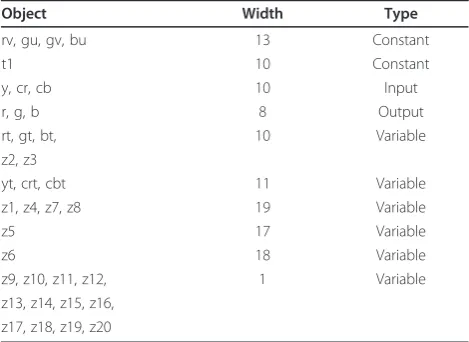
estimated automatically by the synthesis tool or manu-ally by the designer. The bus and register widths com-pletely depend on the object widths. Minimization of the object widths minimizes the total register width in the pipeline under synthesis. For the YCrCb to RGB converter algorithm described in Figure 3, the object, width, and type are given in Table 2.
4.2.4 Longest path delays between operators on acyclic operator precedence graph
The longest path delays between operators constitute a basis for describing pipeline execution time constraints.
We introduce theG matrix that describes the maxi-mum time delays (critical path lengths) between opera-tors on the data flow graph that can be derived from the analysis of the data dependencies between operators and the operator execution times:
G=
⎡ ⎢ ⎣
g1,1· · · g1,n
.. . . .. ...
gn,1· · · gn,n
⎤ ⎥ ⎦,
wheregi, j ati, jÎ Nis a real value. If gi, j= 0, then there exists no path between i and joperators on the data flow graph, and the corresponding element of the
Ptotal matrix is also equal to zero. Ifgi, j> 0, then there is a path between the operators. The Gmatrix can be computed from the vector of operator delays and the
Pdirectmatrix. An algorithm for evaluating longest and shortest path on directed cyclic and acyclic graphs are described in [43].
We present an alternative algorithm for computing the longest path length on DAG, based on the idea that at each step we take an operator for which the longest path lengths of all direct predecessors are evaluated and evaluate the longest path lengths between the taken
operator and all its predecessors in two cases:
1. as a sum of delays of the taken operator and its direct predecessor;
2. as a sum of delay of the taken operator and the longest path length between its direct predecessor and the predecessors of the direct predecessor.
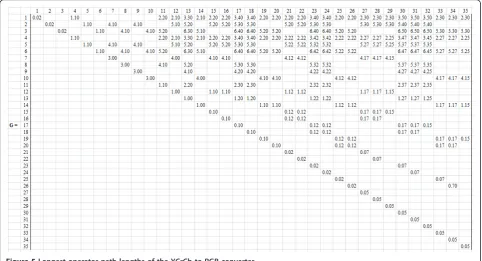
An example of theG matrix for the YCrCb to RGB converter is shown in Figure 5. It should be noted that the longest path between variables may also be used for pipeline synthesis and optimization, in which case a similarGmatrix can be derived. The methodol-ogy in this article considers path length based on operators.
4.2.5 Operator conflict graph
For a given pipelined network, we say thatTstage is its stage time delay, which is the worst time delay of one pipeline stage. Among the pipeline stages, the operator longest path gives maximum stage delay. In the G
matrix of the operator longest paths in the dataflow graph, the valuegi, jmust be less than or equals to Tstage in order for thei andj operators to be included in one stage. If thegi, jvalue is greater than theTstage, then we say that there is a conflict between i and j, and the operators must be scheduled to different stages. Taking such pair of operators, we obtain the operator conflict relation for a given stage delay:
ConflictRelation= (i,j)|i,j∈N and g(i,j)>Tstage
(5)
The operator conflict relation satisfies the requirement as follows:
ConflictRelation⊆PrecedenceRelation (6)
It is obvious that ifTstageis larger than the length of the longest path in the algorithm, thenConflictRelation
=⊘. If the inequalitydelay(i) +delay(j) >Tstageholds for any two adjacent operators i and j on the dataflow graph, then ConflictRelation = PrecedenceRelation. Therefore, the ConflictRelationessentially depends on the value ofTstage. By varying the value ofTstagewe can generate different pipelines for the same dataflow graph description.
The ConflictRelation represents operator conflict directed graph by means of interpreting the pairs(i, j)of operators included in the relation as the graph edges. It should be noted that the conflict graph configuration and the accuracy of the final pipeline synthesis results essentially depend on the accuracy of the operator rela-tive time delay estimation.
Similar to the Gmatrix,variableconflict matrix and graph can also be obtained and used for pipeline synth-esis and optimization.
Table 2 Object width and type in the YCrCb to RGB converter algorithm
Object Width Type
rv, gu, gv, bu 13 Constant
t1 10 Constant
y, cr, cb 10 Input
r, g, b 8 Output
rt, gt, bt, 10 Variable
z2, z3
yt, crt, cbt 11 Variable
z1, z4, z7, z8 19 Variable
z5 17 Variable
z6 18 Variable
z9, z10, z11, z12, 1 Variable
4.2.6 Operator nonconflict graph
By means of subtraction of theConflictRelationfrom the
PrecedenceRelation, we obtain a so-called nonconflict operator relation:
NonConflictRelation=PrecedenceRelation\ConflictRelation (7)
In the relation, a pair(i, j)of operators does not con-stitute a conflict because the operators may be included in the same pipeline stage. For the operators, it is possi-ble thatstage(i) <stage(j), but it is not possible thatstage
(i) >stage(j). The NonConflictRelation varies in the range
∅ ⊆NonConflictRelation⊆PrecedenceRelation (8)
WhenConflictRelationis empty then NonConflictRela-tionequalsPrecedenceRelation. WhenConflictRelationis equal toPrecedenceRelationthenNonConflictRelationis empty.
4.2.7 As soon as possible (ASAP) and as late as possible (ALAP) scheduling
ASAP and ALAP are well-known scheduling techniques that schedule operations in a dataflow graph based on the earliest and latest possible sequence [43]. In this study, we use N set of operators and the
ConflictRelationto generate an ASAP (and ALAP) sche-duling that gives the earliest (and latest) stage that each operator can be scheduled. Tables 3 and 4 show ASAP and ALAP scheduling results for the YCrCb to RGB converter example forTstage= 4.12.
4.2.8 Mobility-based operator ordering
The ASAP and ALAP results give crucial information on the mobility of an operator, which is defined as its possibi-lity to be scheduled to various pipeline stages. We call the earliest stage that an operatorimay be scheduled asasap (i), and the latest asalap(i). Hence, the mobility of opera-toriis given byalap(i)-asap(i). If an operator may be scheduled to only one stage, then the mobility equals to zero. Table 5 shows the mobility of each operator for the YCrCb to RGB converter example forTstage= 4.12. The two non-zero mobility operators, 1 and 4, imply that they can be moved to either pipeline stage-1 or stage-2. The optimization problem is then to determine which of the solutions give optimal results. The next section formulates the optimization problem.
4.3 Pipeline optimization tasks
LetN= {1, ...,n} be a set of algorithm operators andK
= {1, ..., k} be a set of pipeline stages. The number of
Figure 5Longest operator path lengths of the YCrCb to RGB converter.
Table 3 ASAP schedule for the YCrCb to RGB converter for Tstage= 4.12
Stage Operators
1 1, 2, 3, 4, 5, 6, 7, 8, 9, 10
pipeline stages is determined by the stage time delay
Tstage. Variations in the stage delay imply variations in the pipeline stage count. We describe the distribution of operators onto pipeline stages with theXmatrix:
X=
⎡ ⎢ ⎣
x1,1· · · x1,n
.. . . .. ...
xk,1· · · xk,n
⎤ ⎥ ⎦.
In the matrix, the number of rows is equal to the numberkof pipeline stages, and the number of columns is equal to the numbern of operators. A xi, j Î {0, 1} variable for i Î NandjÎ Ktakes one of two possible values. If xi, j = 1, then the ioperator is scheduled to the jstage, otherwise it is not scheduled to the stage. TheX matrix describes a distribution of the operators on the stages.
In some cases, thexi, jvariable can be determined in advance. For example, if 1 ≤ i < asap(j), then xi, j = 0. Similarly,xi, j= 0 foralap(j) <i≤n. Ifi=asap(j) = alap (j), thenxi, j= 1. In order to develop efficient synthesis and optimization techniques, we replace the variables with their known values in theX matrix. The rest of the unassigned variables may be replaced with values 0 or 1 in such a way as to obtain a valid X matrix. One X
matrix describes one possible pipeline schedule. The upper boundSupperof the total number ofXmatrix can be estimated as
Supper=
j∈N
μ(j), (9)
where μ(j) is the number of variables with unknown values in thejcolumn of theXmatrix.
For the YCrCb to RGB converter example with Tstage = 4.12, the asap and alap pipeline stages computed on the operator conflict graph are shown in Figure 6. Operators 1 and 4 may be scheduled to both first and second stages. The other operators are scheduled either to the first stage or to the second stage. The corre-spondingX matrix is presented in Figure 7. Four ele-ments of the matrix are variables (denoted by x), the other elements are constants. The upper bound on the
total number ofX matrix (pipelined schedules) isSupper
= 22= 4. However, actual number of schedules could be less than the upper bound since there are strong depen-dencies among the values of the matrix variables. 4.3.1 Objective function in the optimization task
For a given Tstagerequirement, we can obtain several pipeline schedules. Different schedules give Different parameters. The most important is the number and total width of registers inserted in between neighboring pipeline stages. Minimization of the total register width will save the implementation area. Furthermore, the operating frequency could also possibly be increased with minimization of pipeline registers.
Figure 8 illustrates register usage from pipelining for an example of a 4-stage pipeline. Between the same stage, no registers are used since a particular stage circuit logic is purely combinatorial (indicated by W). Between stage kand k+1, registers are required if an output of an operation in stage kis used in the fol-lowing k+1 stage (indicated by R). If the output of stage kis used by stage k+2 and beyond, then trans-mission registers are required (indicated by T). Our goal is to find the minimum total R and T registers from all possible schedules for a given Ts t a g e constraint.
Let Ω be a set of possible X matrix. For the single-assignment model of the source algorithm, the objective function as follows minimizes the total pipeline register width over all elements of setΩ:
min X∈ k s=1 ⎧ ⎨ ⎩ m j=1 [max
i∈N(fi,j×xs,i)−maxi∈N(hi,j×xs,i)]×width(j)+
m
j=1
[max(τj, max
e=s+1,...,k,i∈N(fi,j×xe,i))−e=smax,...,k,i∈N(hi,j×xe,i)]×width(j)
⎫ ⎬ ⎭,
(10)
whereτj= 1 if thejvariable is an output token andτj = 0 otherwise; × is the arithmetic multiplication operation.
There are two parts in Equation 10. The first one esti-mates for each stagesthe width of registers inserted in between the stage and the previous neighboring stage. The second one estimates for each stage the width of transmission registers.
Table 4 ALAP schedule for the YCrCb to RGB converter for Tstage= 4.12
Stage Operators
1 2, 3, 5, 6, 7, 8, 9, 10
2 1, 4, 11, 12, 13, 14, 15, 16, 17, 18, 19, 20, 21, 22, 23, 24, 25, 26, 27, 28, 29, 30, 31, 32, 33, 34, 35
Table 5 Operator mobility for the YCrCb to RGB converter for Tstage= 4.12
Mobility Operators
0 2, 3, 5, 6, 7, 8, 9, 10, 11, 12, 13, 14, 15, 16, 17, 18, 19, 20, 21, 22, 23, 24, 25, 26, 27, 28, 29, 30, 31, 32, 33, 34, 35
4.3.2 Optimization task constraints
There are three constraints related to our optimization tasks–operator scheduling, time, and precedence constraints.
The operator scheduling constraint describes the requirement that each operator should belong to only one pipeline stage:
alap(i)
s=asap(i)
xs,i= 1 fori∈N, (11)
where sis a pipeline stage from the range asap(i) to
alap(i).
The time constraint describes the requirement that the time delay between two operatorsi andjmust not be larger than Tstage if the operators are scheduled to one pipeline stages:
xs,i×xs,j×gi,j≤Tstage fori,j∈Nands∈K, (12)
wheregi, jis the longest path between iand j opera-tors on the algorithm dataflow graph. It is easy to see that if the operators are in the same stage andxs, i=xs,
j = 1, then the inequality as follows must hold: gi, j ≤
Tstage. If the operators are not in the same stage, then the longest path length may be larger than the stage delay.
The operator precedence constraint describes the requirement that if theioperator is a predecessor of the
joperator on a dataflow graph, then i must be sched-uled to a stage whose number is not greater than the number of stage whichjoperator is scheduled to
alap(i)
s=asap(i) (s×xs,i)−
alap(j)
s=asap(j)
(s×xs,j)≤0for(i,j)∈PrecedenceRelation, (13)
wherePrecedenceRelation⊆N×Nis described by the
Ptotal matrix. Constraints 11, 12, and 13 together define the structure of the optimization space.
4.3.3 Operator conflict and nonconflict directed graphs coloring
The constraints formulated in the previous section describe the rules that must be followed to generate a
valid pipeline schedule. For each pipeline schedule of a givenTstage, acoloring technique is used on the operator conflict and nonconflict graphs to assign an operator to a particular pipeline stage. Reference [43] explains the node coloring technique of anundirected graphG(V, E), which colors the nodes such that no edge (i, j)ÎE, i, j Î V has two end-points with the same color. For any two adjacent nodes i andj, the inequality as follows holds:color(i)≠ color(j). A chromatic number c(G) of the undirected graphGis the minimum number of col-ors over all possible colorings.
However, since our conflict and nonconflict graphs are directed graphs, we introduce coloring on directed
graphs using the following additional requirement: for directed edge (i, j)Î E the inequality as follows should hold:color(i) <color(j). In the pipeline optimization task, if the directed operator conflict graph has a chromatic numberc(G), then the pipeline can be constructed on c (G) stages. We reduce the problem of purely directed graph chromatic number to the problem of longest directed path length in the operator conflict graph. This problem has polynomial complexity.
Node coloring of the YCrCb to RGB converter opera-tor conflict graph is illustrated in Figure 9. The longest node path length equals to 2, therefore the graph chro-matic number c(G) = 2. In this case, two colors are used for the two stages, light and dark colors. Note that nodes 1 and 4 are not colored since they can be colored with either color. However, in order to check which color combinations are valid, the nonconflict graph also needs to be analyzed and colored.
Compared to the operator conflict graph coloring, the operator nonconflict directed graphGn(V, En) is colored in a Different way. The inequality as follows must hold:
max
i∈μin(d)color(i)≤color(d)≤i∈minμout(d)color(i), (14)
wheredÎ V, μin(d) (or μout(d)) is the set of adjacent nodes of dthat are incident toincoming (or outgoing) edges of d. We may also color the nodes from range 1 to c(G), where c(G) is the chromatic number of the operator conflict graph. The only restriction in such
Figure 6ASAP and ALAP pipeline stages for the scheduled operators for the YCrCb to RGB converter example withTstage= 4.12.
coloring is thatcolor(i)may not be larger thancolor(j) if (i, j)ÎEn. Moreover, the nonconflict graph enables col-oring the nodes that are not colored in the conflict graph.
Going back to the example, we can now color nodes 1 and 4 with either one of the following: node 1 with light color and node 4 with light color; node 1 with light color and node 4 with dark color; node 1 with dark color and node 4 with dark color. Note that as revealed in the nonconflict graph in Figure 10, the coloring of node 1 with dark color and node 4 with light color is not valid.
5 Pipeline synthesis and optimization methodology and algorithms
This section presents methodology and key algorithms for our pipeline synthesis and optimization technique. Based on the formulations described in Section 4, a pro-gram was developed in Java under the Eclipse IDE that transforms a non-pipelined CAL actor into pipelined CAL actors.
The general overview is given in Figure 11. Starting from a non-pipelined CAL actor, the matricesF, H, P dir-ect,Ptotal, andGas well as the list [Tmin, ...,Tmax] of the possible stage timeTstagevalues are computed. TheTmin
value equals the operator highest execution time, and the
Tmaxvalue equals the longest path weight in actor data-flow graph. Optimization of pipelines is performed in a loop on various stage numbers. We start with one-stage pipeline (K= 1) and stage timeTstage=Tmax. For the cur-rentTstage, the conflict and nonconflict operator relations and directed graphsGcandGncare generated from the
Gmatrix andPtotalrelation. The chromatic number of the graphs is computed using a polynomial complexity algorithm. If the chromatic number is larger than the stage numberK, then the successor value of Tstage is taken in the ascending list of stage time values. Owing to this, we use the lowest value ofTstagefor each numberK of stages and thus generate the fastestK-stage pipeline. If the chromatic number is larger than the stage numberK, then the predecessor value ofTstagein the list is taken as its current value ifTstage>Tmin, and0is taken otherwise. If for the updated valueTstage<Tmin, then the optimiza-tion result is a set of pipelined networks of CAL actors for various stage numbers. Otherwise, the conflict and nonconflict graphs are generated again for an updated value ofTstage. In order to evaluate the operator mobility and to perform the critical path-based arrangement of graph colorings, the ASAP and ALAP schedules are gen-erated. We propose ordered vertex coloring to order the
generation of solutions. The vertices in the critical (long-est) paths are colored first. Owing to this approach, pre-ferable solutions are generated first. Among them, the best (optimal or proximate) solution is selected using the pipeline register total width estimated with Equation 10. The best solution is generated with a branch and bound algorithm and finally used to generate pipelined CAL actors which are then synthesized to HDL for FPGA implementation.
In the remainder of this section, key algorithms for generating valid operator colorings on the conflict and nonconflict directed graphs and searching for an optimal pipeline schedule will be presented.
The technique for generating various operator color-ings is based on recursive function and explicit stack mechanism. Figure 12 shows a top level recursive func-tion Reg-WidthColoringStep which is used to generate pipeline schedules, and minimize the total pipeline reg-ister width. The algorithm takes in three inputs:
1.asap, which is an array of operators with the cor-responding pipeline stage using the ASAP algorithm; 2.alap, which is an array of operators with the cor-responding pipeline stage using the ALAP algorithm; 3. order, which is an array of operators ordered according to its mobility over pipeline stages;
and generates the following output:
1. pipelineCount, which is the number of generated pipelines;
2.optimalColor, which is the optimal pipeline sche-dule as an array of operators with the corresponding pipeline stage;
3.minRegWidth, which is the minimum total register width of the optimal pipeline schedule.
The algorithm in Figure 12 works as follows. The recursive function takes in an input parameter top, which indicates the top record in the stack of operators.
Depending on thetopvalue, the function can return the control, generate the next complete coloring solution and compare it with the best current one, choose the next correct color of the current operator and generate the next record in the stack for procedure recursive call. In the nexttop+1 record, the minimum and maximum colors of the next operator are determined. If the mini-mum color is larger than the maximini-mum color, then recoloring of the current operator is performed. The computations of minimum and maximum colors for operators are performed for both the conflict and the nonconflict graphs.
Figure 13 shows an algorithm to estimate minimum colors from a conflict graph. Among all operators that are recorded in the stack as predecessors and are in conflict relation with the given operatorop, the operator
with maximum color gives the value of minC that is returned by the algorithm as minimum color of op
operator. The computations of maximum color from a conflict graph, minimum color from a nonconflict
graph, and maximum color from a nonconflict graph are performed in a similar way. Once all operators have been colored and a valid pipeline schedule is generated, the total register width is estimated to evaluate the effi-ciency of the schedule. The functiontotalRegister-Width (colors) performs this, which takes in a pipeline sche-dule, and returns the total register width. The function sums the width of all required pipeline and transmission registers of a pipeline schedule. From all possible pipe-line schedules, the smallest total register width is stored in the variable minRegWidthwith the corresponding
optimal-Colorsas the best schedule.
The final step is to generate CAL actors from the optimal coloring. This is done by taking the optimalCo-lors array, partition the operators according to the scheduled stage, and print the required operations, vari-ables, registers, inputs, and outputs declarations accord-ing to the syntax of the CAL dataflow language. The top levelXDFnetwork of pipelined CAL actors is also auto-matically generated based on the required number of pipeline stages.
It should be noted that our program is designed to generate potentially all possible valid pipeline schedules for a given Tstageconstraint, therefore results in a global optimum solution. The number of possible schedules depends on the mobility of operators; an algorithm with many operators that can be moved among various stages would generate many possible schedules, therefore could potentially take a long time to find a global optimum. The RegWidthColoringStep function is a basic one for creating modifications which would restrict the number of generated solutions. Thus, it is modified to a branch-and-bound algorithm by means of introducing a
RegWidthLowerBound function, which estimates a lower bound of total pipeline register width using partial operator coloring that is recorded in the stack, and ASAP and ALAP colorings. The number of generated solutions is also restricted with MeetOptimizationTime-Constraintfunction which takes into account the spent CPU time or the number of produced partial and com-plete colorings.
6 Experimental results
This section presents experimental results of our pipe-line synthesis and optimization technique. Three video processing algorithms with relatively large combinatorial logic are selected for pipelining–they are the YCrCb to RGB converter, 8 × 8 1D IDCT, and Bayer filter. It is assumed that these algorithms constitute a critical path in a larger design, therefore, by pipelining these algo-rithms, a throughput increase can be obtained for the overall system.
Each design starts with an initial single CAL actor description, automatically pipelined using our tools to
obtain multiple-actor description, and synthesized to HDL. For hardware implementation, two different 65-nm process node FPGAs have been used; Xilinx Virtex-5 and Altera Stratix III, synthesized using Xilinx XST and Altera Design Compiler tools, respectively.
6.1 YCrCb to RGB converter based on Xilinx XAPP930 [42]
This design was introduced in Section 3.2 for illustrating our methodology. A single actor was constructed that converts YCrCb to RGB color space. The total number of operators is 35.
The first step is to analyze validTstage constraints by determining the minimum and maximumTstagefrom the dataflow graph (Figure 4). This is done by looking at Table 1 for estimating the delay of operators. From the dataflow graph, the minimumTstage is defined by the multiplication operator which is equals to 3.00. The max-imumTstageis defined by the longest path length, given in Figure 5 which is 6.50. As a result, aTstageconstraint of 3.00 synthesizes to a 3-stage pipeline, while a stage delay of 6.50 and above gives a non-pipelined implemen-tation. Further analysis of the dataflow graph shows dependency of the multiplication operators to the pre-vious operations of bitand and subtraction. Therefore, a
Tstageof 4.12 (bitand-subtract-multiply) is the minimum for which the pipeline would synthesize to 2-stages.
Figure 14 shows a graph of number of pipeline stages versus Tstageconstraint. Tstagespecification of between 3.00 and 4.12 synthesizes to a 3-stage pipeline, between 4.12 and 6.50 to a 2-stage pipeline, and 6.50 and above gives a 1-stage pipeline (i.e. non-pipelined) to obtain best performance for a particular number of pipeline stages, the minimumTstageshould be selected.
The results for 2-stage and 3-stage pipelines are given in Table 6. ForTstage= 4.12 with a synthesis to 2-stage pipeline, the optimal schedule (best) results in total reg-ister width of 83, while in the worst case, total regreg-ister width is 92. This results in 10.8% reduction in total reg-ister width. For Tstage = 3.00 with a synthesis to 3-stage pipeline, minimum total register width is 122 compared to 131 in the worst case, with a reduction of 7.4%. Note that reduction of register widths between best and worst case are relatively small because of the limited optimiza-tion space for this example, with just three for each pipeline stages.
registers and LUTs. In terms of throughput, the opti-mized 2-stage and 3-stage pipelines are roughly 65% higher compared to a non-pipelined implementation. As for Stratix III, a slightly different result is observed. Similar to Virtex-5, there is a very little difference in resource between the best and the worst case pipelines. Compared to a non-pipeline implementation, 2-stages pipeline utilizes roughly 22% more ALUT, with 59% higher throughput. For the 3-stage pipeline, ALUT is increased by up to 44% with 57% more throughput.
In both FPGAs, it can be seen that the throughput is almost similar for 2-stages and 3-stages pipeline imple-mentations. In other words, 3-stage pipeline does not result in significant increase in throughput compared to a 2-stage pipeline. The reason is due to the saturation of
throughput, because at this point, the critical path is now in the control (i.e. registers) and hardware inter-connection rather than the operators as in the non-pipe-lined implementation.
It should be noted that the ASAP and ALAP pipeline schedules can also be generated and compared. However, because of the small optimization space of this design, the ASAP pipeline schedule is found to be the same as the worst case schedule, and ALAP to be the same as the best case schedule. The next two examples present designs with significantly larger optimization space.
6.2 8 × 8 1D IDCT based on ISO/IEC 23002-2 [44]
The IDCT, or the Inverse Discrete Cosine Transform, is used in almost all image and video decompression
R e g W i d t h C o l o r i n g S t e p ( t o p ) b e g i n
i f t o p >= n t h e n
c o m p l e t e C o l o r i n g s := c o m p l e t e C o l o r i n g s + 1 ; regWidth := t o t a l R e g i s t e r W i d t h ( C o l o r S t a c k ) ;
i f minRegWidth > regWidth t h e n
o p t i m a l C o l o r s := c o l o r S t a c k ; minRegWidth := regWidth ;
i f n o t M e e t O p t i m i z a t i o n T i m e C o n s t r a i n t ( ) t h e n e x i t ;
end i f
r e t u r n ;
end i f
f o r c i n m i n C o l o r ( t o p ) t o maxColor ( t o p ) do
c o l o r S t a c k ( t o p ) := c ;
i f RegWidthLowerBound ( c o l o r S t a c k , asap , a l a p ) >= minRegWidth t h e n
c u t B r a n c h e s := c u t B r a n c h e s + 1 ; c o n t i n u e ;
end i f
i f t o p < n−1 t h e n
o p e r := o r d e r ( t o p + 1 ) ;
minC := e s t i m a t e M i n C o n f l i c t C o l o r ( C o l o r S t a c k , top , o p e r , C o n f l i c t R e l a t i o n ) ; maxC := e s t i m a t e M a x C o n f l i c t C o l o r ( C o l o r S t a c k , top , o p e r , C o n f l i c t R e l a t i o n ) ; minP := e s t i m a t e M i n N o n C o n f l i c t C o l o r ( C o l o r S t a c k , top , o p e r ,
N o n C o n f l i c t R e l a t i o n ) ;
maxP := e s t i m a t e M a x N o n C o n f l i c t C o l o r ( C o l o r S t a c k , top , o p e r , N o n C o n f l i c t R e l a t i o n ) ;
m i n C o l o r ( t o p +1) := maximum ( a s a p ( o r d e r ( t o p + 1 ) ) , minC+1 ,minP ) ;
maxColor ( t o p +1) := minimum ( a l a p ( o r d e r ( t o p + 1 ) ) ,maxC−1 ,maxP ) ;
i f m i n C o l o r ( t o p +1) > maxColor ( t o p +1) t h e n c o n t i n u e ; end i f
end i f
c o l o r i n g S t e p ( t o p + 1 ) ;
end f o r
end
Figure 12The algorithm of register width minimization on set of operator colorings.
e s t i m a t e M i n C o n f l i c t C o l o r ( C o l o r S t a c k , top , op , C o n f l i c t R e l a t i o n ) b e g i n
minC := 0 ;
f o r i i n 0 t o t o p do
c := c o l o r S t a c k ( i ) ; nd := o r d e r ( i ) ;
i f ( nd , op ) i s i n C o n f l i c t R e l a t i o n t h e n
i f minC < c t h e n minC := c ; end i f
end i f
end f o r
r e t u r n minC ; end
standard, for example in classical JPEG, MPEG-1, MPEG-2, MPEG-4, H.261, H.263, and JVT (H.26L) [45]. The reason for this is because of the strength of its inverse, the DCT, in which images are coded with inter-pixel redundancies, therefore offers excellent de-correla-tion for most natural images. The DCT also packs energy in the low frequency regions, which allows the removal of high frequency regions without significant quality degradation.
Image and video decompression systems use two-dimensional (2D) version of the IDCT, which is two one-dimensional (1D) IDCTs arranged serially with a transpose memory element in between. In the context of RTL, the two 1D IDCTs are normally treated as sepa-rate entities; therefore, the critical path is defined as the longest path of a 1D IDCT. For a parallel implementa-tion of the 1D IDCT with large combinatorial logic, pipelining is an interesting strategy for improving data throughput.
Recently, the international standard organizations, ISO/IEC released the 23003-2 standard for coding and decoding MPEG video technology using fixed-point 8 × 8 IDCT and DCT. Among others, it pro-vides approximation methods to ease implementation of codecs, ensure that the codecs are implemented in full conformance to specification, specifies single deterministic results as the output of an image or video encoding and decoding process, and improve the quality of delivered video and image representations.
Figure 17 shows the dataflow graph of the 23002-2 8 × 8 1D IDCT in a single-assignment form. The algo-rithm uses 25 subtractors and 19 adders, where we assumed the same delay of 1.00 for both the operators. It takes in eight inputs in parallel (i.e. one line of an 8 × 8 block), and produces eight parallel outputs. All vari-ables are set to 26 bits, including input and output ports. The total number of variables is 52. The algo-rithms also use 21 shifters, which are not considered in the dataflow graph, since this element is considered to have no cost in the context of RTL.
The first step is to determine validTstageconstraints by finding the largest single operator delay (minimum
Tstage) and longest path length (maximum Tstage). Since the algorithm consists of only adders and subtractors, the minimum Tstage is found to be 1.00. The longest path length is found by analyzing the dataflow graph, which is 7.00. As shown in Figure 18, a Tstage = 1.00 synthesizes to a 7-stage pipeline,Tstage= 2.00 to a 4-stage pipeline,Tstage= 3.00 to a 3-stage pipeline, Tstage
Figure 14Number of pipeline stages (Nstage) versus stage-delay (Tstage) for the YCrCb to RGB converter.
Table 6 The YCrCb to RGB converter: exploration of pipeline optimization space
Nstage 2 3
Tstage 4.12 3.00
Reg-width best 83 122
Reg-width worst 92 131
Reg-width reduction (%) 10.8 7.4
= 4.00 to a 2-stage pipeline, and Tstage ≥ 7 to a non-pipelined implementation.
For each of the n-stage pipeline for n = {2, 3, 4, 7}, ASAP, ALAP, best, and worst schedules are generated.
Table 7 summarizes the result. For a 2-stage pipeline of
Tstage = 4.00, the highest total register width is the worst-case with 494, followed by ASAP with 364, ALAP with 312, and the best case with only 260. This results
Figure 15Slice versus throughput for all implementations of the YCrCb to RGB converter for Xilinx Virtex-5.
in a register-width reduction of 90% compared to the worst-case. The optimization space for this pipeline con-figuration is 24, 336. For a 3-stage pipeline, register width reduction between best and worst cases is almost similar, with 88.9%. However, the optimization space is significantly more with 29, 555, 604 possible pipeline schedules. The 4-stage design shows the highest number of optimization space with more than 63 million sche-dules, with register width reduction of 43.8%. The smal-lest reduction is in the 7-stage pipeline with only 21.9%. This configuration also results in the most total register
width with up to 2, 028 in the worst case. For this example, although the number of feasible schedules is large, our branch and bound algorithm generated only 5, 3, 1, and 1 complete colorings (schedules) for 2, 3, 4, and 7 pipeline stages, respectively, and cut all other branches in the search tree.
All designs have been synthesized to HDL, and then to Xilinx Virtex-5 and Altera Stratix III FPGAs for implementation. The results are shown in Figures 19 and 20. For Virtex-5, non-pipeline implementation results in 1, 650 total slice with throughput of 764
Mpixels/s, while for Stratix III, it utilizes 1, 571 ALUT with throughput of 922 Mpixels/s. In both FPGAs, resource and throughput show nearly a linear increase from 2-stages to 4-stages pipeline. However, the throughput of 7-stage pipeline for Virtex-5 saturates at roughly the throughput of 3-stages and 4-stages pipe-line, while this is not the case for Stratix III. The maxi-mum throughput using Virtex-5 FPGA is 1654 Mpixels/ s with total slice of 3, 419 for 4-stages pipeline, which corresponds to 2.07× more slice and 2.16× higher
throughput compared to non-pipeline implementation. However, for the best case (resource optimized) 4-stages pipeline, it utilizes only 70% more slice with a through-put increase of 2.08×. As for Stratix III, the highest throughput is the optimal solution (i.e. least resource) for a 7-stage pipeline with 2457 Mpixels/s and ALUT of 3632, which corresponds to 2.31× more ALUT and 2.66× higher throughput. However, higher throughput-to-resource ratio can be obtained in the 4-stages pipe-line with only 56% more ALUT and throughput increase by 2.38× compared to non-pipeline implementation. At this level as well (4-stages pipeline), the worst-case design utilizes 15% more ALUT compared to the opti-mal solution.
6.3 Bayer filter based on improved linear interpolation [46]
Bayer filter is commonly used for demosaicing of color images produced by single-CCD (charge-coupled device) digital cameras. The CCD pixels are preceded in the optical path by a color filter array in a Bayer mosaic pat-tern, where for each set of 2 × 2 pixels, two diagonally opposed pixels have green filters, and the other two
Figure 18Number of pipeline stages (Nstage) versus stage-delay (Tstage) for the 8 × 8 1D IDCT.
Table 7 The 8 × 8 1D IDCT: exploration of pipeline optimization space
Nstage 2 3 4 7
Tstage 4.00 3.00 2.00 1.00
Reg-width asap 364 520 832 1664
Reg-width alap 312 624 832 1716
Reg-width best 260 468 832 1664
Reg-width worst 494 884 1196 2028
Reg-width reduction (%) 90.0 88.9 43.8 21.9
Feasible schedules 24336 29555604 63002926 4505752
Cut branches 592 1803470 12295281 1298947
have red and blue filters. The green component is sampled at twice the rate of red and blue since it carries most of the luminance information. The Bayer filter interpolates back the image captured by the CCD
sensor, so that every pixel from the sensor (RGGB) can be associated to a full RGB value.
There exists several techniques and algorithms to interpolate images from a CCD sensor. Recently, a new
Figure 19Slice versus throughput for all implementations of the 8 × 8 1D IDCT for Xilinx Virtex-5.
interpolation technique was introduced [46] that outper-forms other linear and non-linear algorithms in terms of performance and complexity, and results in high quality output image. In this example, we implemented this technique using the CAL dataflow program, and use our pipeline synthesis and optimization program to find the best pipelining strategy for this design.
The dataflow architecture of the bayer filter has been designed using three separate actors; the cache, core, andcontrol. Thecache simply stores the incoming data up to the fifth row, since the core image filtering is done on a 5 × 5 kernel size. Thecore then takes in each
kernel, performs image convolution using pre-deter-mined constant coefficients, and outputs the filter core parametersbtr, gtr, rtg, andbtg. Thecontrol keeps track of the current location as to output the correct RGB value. For example, if the current location of the sensor is on the blue pixel, then the control simply setsr = btr, g = gtr, and b = center, where center is the blue pixel from the sensor.
From these three actors, the main computation and processing is in the core. Therefore, pipelining this actor is key to obtaining a higher throughput system. The core takes in 13 parallel 8-bit input from a 5 × 5 kernel
to generate the core outputs. The dataflow graph of the core is shown in Figure 21. The inputs are x0to x12. The algorithm requires 13 bitands, 20 subtractors, 31 adders, 3 multipliers, and 25 shifters. Similar to the IDCT, shifters are not included in the dataflow graph as it is assumed to have no cost for FPGA implementation. The first step is to determine the range for validTstage. For this example, we use the operator delays as given in Table 1. The minimumTstageis determined by the mul-tiply operator, which is 3.00 that would synthesize to the maximum number of pipeline stagesNstage= 7. The maximumTstageis found from the longest path matrix
G, which is 15.62. Any value greater than this would synthesize to a non-pipelined implementation. Further
analysis of the dataflow graph shows that for a 2-stage pipeline, minimum Tstage is 8.30, 3-stage pipeline for
Tstage= 5.32, 4-stage pipeline for Tstage = 4.30, 5-stage pipeline forTstage= 3.22, and 6-stage pipeline forTstage = 3.10. The graph ofNstage versusTstage is given in Fig-ure 22.
For each Nstagegiven in Figure 22, the optimization space is explored for ASAP, ALAP, best, and worst pipe-line schedules. Table 8 summarizes the result. For 2-stage pipeline with Tstage = 8.30, the largest register width reduction (156%) is achieved for optimization space of 1440. In this case, the best register width is 147, while the worst is 376. Moving to the 3-stage pipe-line, there is still a significant register width reduction of 94.0% from 660 in the worst case to 340 in the best case. For 4-stages and above, the optimization space is too large (> 1010), therefore, only 108schedules are gen-erated to find the best proximate solution. Nevertheless, results show significant register width reduction of 108.0, 94.1, 69.8, and 94.1%, respectively, for 4, 5, 6, and 7 stages pipeline.
All the best solutions also show superior results com-pared to ASAP and ALAP schedules by significant mar-gins. Compared to ASAP the reduction in the total pipeline register width is 46.2, 33.2, 51.3, 46.8, 29.5, and 30.4% for 1 to 7 stages pipelines. In average, the reduc-tion is 39.6%. Similarly for ALAP, the reducreduc-tion in the
Figure 22Number of pipeline stages (Nstage) versus stage-delay (Tstage) for the bayer filter core.
Table 8 The bayer filter core: exploration of pipeline optimization space
Nstage 2 3 4 5 6 7
Tstage 8.30 5.32 4.30 3.22 3.10 3.00
Reg-width asap 215 453 737 998 1259 1428
Reg-width alap 308 501 710 949 1273 1383
Reg-width best 147 340 487 680 972 1095
Reg-width worst 376 660 1013 1320 1650 1658
Reg-width reduction (%)
156.0 94.0 108.0 94.1 69.8 51.4
Feasible schedules 1440 264384 >
1010 > 1010
> 1010
Figure 23Slice versus throughput for all implementations of the bayer filter core for Xilinx Virtex-5.