Evaluation of different approaches to individual tree growth and survival modelling using data collected at irregular intervals – a case study for Pinus patula in Kenya

(1)

R E S E A R C H A R T I C L E

Open Access

Evaluation of different approaches to individual

tree growth and survival modelling using data

collected at irregular intervals

–

a case study for

Pinus patula

in Kenya

Rita Juma

1

, Timo Pukkala

1*

, Sergio de-Miguel

1

and Mbae Muchiri

2

Abstract

Background:The minimum set of sub-models for simulating stand dynamics on an individual-tree basis consists of tree-level models for diameter increment and survival. Ingrowth model is a necessary third component in uneven-aged management. The development of this type of model set needs data from permanent plots, in which all trees have been numbered and measured at regular intervals for diameter and survival. New trees passing the ingrowth limit should also be numbered and measured. Unfortunately, few datasets meet all these requirements. The trees may not have numbers or the length of the measurement interval varies. Ingrowth trees may not have been measured, or the number tags may have disappeared causing errors in tree identification.

Methods:This article discussed and demonstrated the use of an optimization-based approach to individual-tree growth modelling, which makes it possible to utilize data sets having one or several of the above deficiencies. The idea is to estimate all parameters of the sub-models of a growth simulator simultaneously in such a way that, when simulation begins from the diameter distribution at the first measurement occasion, it yields a similar ending diameter distribution as measured in the second measurement occasion. The method was applied toPinus patula permanent sample plot data from Kenya. In this dataset, trees were correctly numbered and identified but measurement interval varied from 1 to 13 years. Two simple regression approaches were used and compared to the optimization-based model recovery approach.

Results:The optimization-based approach resulted in far more accurate simulations of stand basal area and number of surviving trees than the equations fitted through regression analysis.

Conclusions:The optimization-based modelling approach can be recommended for growth modelling when the modelling data have been collected at irregular measurement intervals.

Keywords:Model recovery; Stand dynamics; Observational plots; Permanent sample plots

Background

The most flexible growth model type in irregular and mixed stands is a set of individual tree models, consisting of separate models for different species or species groups, or using indicator variables for species-specific growth patterns. Individual-tree models may be the best overall tool for predicting the dynamics of tree stands. Stand-level models may be more reliable in even-aged plantations but

they may encounter problems in uneven-aged and mixed stands. The minimum set of sub-models for simulating stand development consists of individual-tree models for diameter increment and survival. Tree height, volume and biomass may be calculated with static models. If uneven-aged management is an option, a necessary third compo-nent is a model for ingrowth or regeneration.

The development of this type of model set needs data from permanent plots, in which all trees have been num-bered and tagged, and measured at regular intervals for diameter and survival. New trees passing the ingrowth * Correspondence:[email protected]

1_{University of Eastern Finland, PO Box 111, Joensuu 80101, Finland}

Full list of author information is available at the end of the article

(2)

limit (i.e., the minimum measured diameter) between two measurement occasions should also be tagged, num-bered and measured. Unfortunately, these requirements are not always met. There may be plenty of data, but their use in individual-tree modelling is complicated for instance due to the following reasons:

Trees have not been numbered. The data may be error-free but growth and survival information is not available for individual trees.

There are many tree-identification errors. This may happen for instance when tree identification is based on a certain measurement order of trees. Mortality and ingrowth may make it difficult to keep the same order in successive measurements, leading to situations in which the sequences of tree-level measurements are not always from the same tree.

Measurement interval varies, making it difficult to develop a growth model for a certain time step (e.g. 1 year or 5 years).

Pukkala et al. (2011) proposed an optimization-based method, which can be used to recover individual-tree models using data in which individual trees are not iden-tified. All parameters of the sub-models of a growth simulator were recovered simultaneously in such a way that the simulated stand development, when started from the initial diameter distribution, yielded the measured ending distribution. The parameters of the diameter incre-ment, survival and ingrowth models for three different species were recovered simultaneously. The data came from the permanent plots of several silvicultural experi-ments where the tree diameters were measured accurately but the trees were not tagged or numbered. This made it impossible to calculate the growth and survival of indi-vidual trees or identify ingrowth trees. The measure-ment interval was not constant. Despite these problems, Pukkala et al. (2011) were able to develop ingrowth models for different species, as well as individual-tree models for diameter increment and survival. The used methodology was tested in another dataset in which the measurement interval was constant, trees had number tags, and ingrowth trees were identified and numbered. In this dataset, the optimization-based recovery approach yielded models that were very similar to ordinary regres-sion models.

The same method was used by de-Miguel et al. (2014) to develop individual-tree diameter increment and survival models for balsa (Ochroma pyramidale) plantations in Bolivia. The data came from permanent plots. The purpose was to measure the trees always in the same order, which seemed easy because trees were planted in straight rows. However, high mortality rate typical to balsa resulted in a data set in which successive diameter recordings did not

always represent the same tree. Tree identification errors were many, making it almost impossible to derive diameter increment and survival models by using ordinary regres-sion analysis techniques. Yet, by using the optimization-based recovery technique, de-Miguel et al. (2014) were able to develop plausible models for one-year diameter incre-ment and tree survival in balsa plantations. The researchers tested the method using accurate data on another tropical plantation species, tejeyeque (Centrolobium tomentosum) (de-Miguel et al. 2013). The comparison showed that optimization resulted in models that were very similar to models fitted in regression analysis. In prediction, optimization-based models performed better than mar-ginal and conditional predictions of mixed-effects models, and were almost as good as fixed-effects models.

The impact of irregular measurement interval on mod-elling has received some attention in earlier research (Cao 2000 2004; Nord-Larsen 2006; Crecente-Campo et al. 2010). Assuming a constant growth between measure-ments can lead to under- and over-estimation of tree growth when growth dynamics are clearly nonlinear (Clutter 1963; McDill and Amateis 1992). McDill and Amateis (1992) suggested the use of correction factors that force the interpolated growths to be consistent with the estimated growth function. Cao (2004) proposed an iterative technique, in which the calculation of the in-terim values of stand level predictor variables was based on stand-level models. The approach of Nord-Larsen (2006) places tree survival at the end of the growth period. Therefore, the effect of gradual mortality on the interim values of tree- and stand-level competition vari-ables is ignored. Crecente-Campo et al. (2010) used re-peated fittings and simulations with the fitted models to calculate the interim values of predictors. Mortality was simulated by assuming that those trees will die that have the predicted survival probability less than an iteratively found threshold value.

Pinus patulais the most intensively utilized conifer in the tropics and sub tropics, where it is widely planted as an exotic (Wright 1994). The species is native to Mexico (Dvorak and Donahue 1992; Dvorak et al. 2000).

P. patula has been introduced for instance to South Africa, Swaziland, Zimbabwe, Madagascar, Malawi, Tanzania, Kenya, Uganda, Angola and Cameroon (Wormald 1975). The plantations occur over a wide range of sites of varying productive potential and are of major im-portance in these regions (Record and Hess 1974; Isango and Nshubemuki 1998; Mabvurira and Musokonyi 1998; Muchiri and Muturi 1998).

(3)

tannins. They also produce fuel-wood and raw material for charcoal. The plantations also play a role in the protec-tion of watershed areas and restoraprotec-tion of degraded land (Palmer and Gibbs 1974).P. patulais also planted in wind-breaks, as a shade tree for coffee and as an ornamental tree. The current area of P. patula plantations in Kenya is about 100,000 ha (Muchiri and Muturi 1998). Despite its importance, no individual-tree growth models have been developed for Kenyan P. patulaplantations. One reason for this situation is that, although there are permanent plot data in Kenya, they have not been measured system-atically making the available data difficult to be used in modelling.

This study applied the optimization-based parameter recovery technique for P. patula plantations in Kenya. Trees have been carefully numbered and measured re-peatedly in several plots during a 30-year period. The dataset is valuable since it covers the whole rotation period. The problem with the data is irregular measure-ment interval, ranging from 1 to 13 years. Two other ap-proaches to deal with irregular measurement intervals were tested and compared with the optimization-based approach. The optimization-based method was used for the first time to recover mixed-effects models.

Methods Experiment

The data used in this study were collected from aP. patula

experiment established in 1967 in Londiani Forest Station

in Kericho County of Rift Valley province, situated at approximately latitude 0° 05’ S and longitude 35°53’ E at an altitude of 2,300–2,400 m above sea level. The area receives a mean annual rainfall of about 1,200 mm with a bimodal distribution pattern with long rains oc-curring between March and June, and the short rains between mid September and November (Jaetzold and Schmidt 1983). The mean annual temperature is 18°C with a maximum of 24°C.

The P. patula permanent sample plots were primarily established to observe the effect of stocking onP. patula

growth. The study area consists of four randomized blocks with seven different spacings per block, resulting in 28 plots of 0.059 ha each. The plan was to measure diameter at breast height, diameter at ground level, tree height and survival annually from age 7 to 14 (1974–1980), followed by every 3 years up to the age of 19 years, and afterwards every 5 years up to rotation age of 30 years. However, the plan was not followed rigorously, and the actual interval varied from 1 to 13 years. The number of measurements in the same plot was 7–10, resulting in 6–9 periods per plot. However, since the measurement years were not al-ways the same for all plots, the total number of periods was 13. The last measurement was conducted in 1996. At each measurement, tree diameter at 1.3 m height (dbh) for all trees, and tree heights of a sample of at least 8 trees per plot were recorded. This resulted in 13,483 diameter increment observations and 1,698 height observations (Table 1). Trees sampled for height were not necessarily

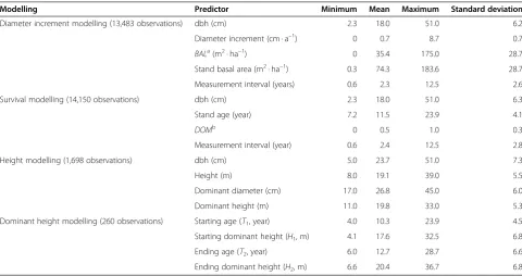
Table 1 Descriptive statistics of the modelling data

Modelling Predictor Minimum Mean Maximum Standard deviation

Diameter increment modelling (13,483 observations) dbh (cm) 2.3 18.0 51.0 6.2

Diameter increment (cm · a–1₎ ₀ _0.7 _8.7 _0.7

BALa_(m2_{· ha}–1₎ ₀ _35.4 _175.0 _28.7

Stand basal area (m2_{· ha}–1₎ _0.3 _74.3 _183.6 _28.7

Measurement interval (years) 0.6 2.3 12.5 2.6

Survival modelling (14,150 observations) dbh (cm) 2.3 18.0 51.0 6.3

Stand age (year) 7.2 11.5 23.9 4.1

DOMb ₀ _0.5 _1.0 _0.3

Measurement interval (year) 0.6 2.4 12.5 2.8

Height modelling (1,698 observations) dbh (cm) 5.0 23.7 51.0 7.3

Height (m) 8.0 19.1 39.0 5.5

Dominant diameter (cm) 17.0 26.8 45.0 6.0

Dominant height (m) 11.0 19.8 33.0 5.3

Dominant height modelling (260 observations) Starting age (T1, year) 4.0 10.3 23.9 4.5

Starting dominant height (H1, m) 4.1 17.6 32.5 6.8

Ending age (T2, year) 6.0 12.7 28.7 6.6

Ending dominant height (H2, m) 6.6 20.4 36.7 6.8

a

Basal area in larger trees. b

(4)

the same in different measurements. Dead trees were re-corded at each measurement.

Height modelling

A model for dominant height development along age was fitted for site index calculations. Dominant height was de-fined as the average height of 100 largest (in terms of dbh) trees per hectare. To calculate dominant height, a plot-wise measurement-specific diameter-height model was fitted and used to calculate the heights of trees that were not measured for height.

Several different equation forms (Peschel 1938; Schumacher 1939; Lundqvist 1957; Richards 1959; Sloboda 1971; McDill and Amateis 1992; Diéguez-Aranda et al. 2005, 2006) derived by using either algebraic ferential equations (ADA) or generalized algebraic dif-ferential equations (GADA) (Bailey and Clutter 1974; Cieszewski and Bailey 2000) were tested as candidate models for modelling dominant height growth. The se-lected model was used to estimate the site index of each plot using 30 years as index age.

All individual-tree height observations were used to fit an individual tree height model. Several variants of the model based on Stoffels and van Soest (1953) modified

by Tomé (1989) were tested in height-diameter modelling. Tree height was predicted from tree diameter, dominant height and dominant diameter. The used model form guarantees that the simulated height development of indi-vidual trees is logically related to the dominant height de-velopment of the stand.

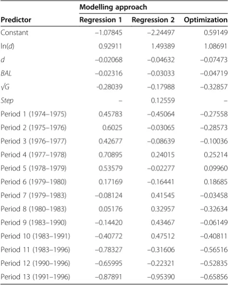
Table 2 Coefficients of the mixed-effects diameter increment models

Modelling approach

Predictor Regression 1 Regression 2 Optimization

Constant –1.07845 –2.24497 0.59149

ln(d) 0.92911 1.49389 1.08691

d –0.02068 –0.04632 –0.07473

BAL –0.02316 –0.03033 –0.04719

√G -0.28039 –0.17988 –0.32857

Step – 0.12559 –

Period 1 (1974–1975) 0.45783 –0.45064 –0.27558

Period 2 (1975–1976) 0.6025 –0.03065 –0.28573

Period 3 (1976–1977) 0.42677 –0.08639 –0.10036

Period 4 (1977–1978) 0.70895 0.24015 0.25214

Period 5 (1978–1979) 0.53579 –0.02277 0.09960

Period 6 (1979–1980) 0.17169 –0.16441 0.18685

Period 7 (1979–1983) –0.08124 0.41545 –0.03458

Period 8 (1980–1983) 0.05176 0.32957 –0.32634

Period 9 (1983–1990) –0.14420 0.43467 –0.06149

Period 10 (1983–1991) –0.40772 0.47512 –0.40811

Period 11 (1983–1996) –0.78327 –0.31606 –0.56516

Period 12 (1990–1996) –0.65995 –0.22321 –0.52835

Period 13 (1991–1996) –0.87891 –0.95390 –0.65856

d= diameter at breast height;BAL= basal area in larger trees;G= stand basal area.

Table 3 Regression coefficients of the mixed-effects survival models

Predictor

Modelling approach

Regression 1 Regression 2 Optimization

Constant 2.81439 6.42965 6.42705

ln(d) 2.96858 3.35703 1.83056

d –0.08303 –0.08219 –0.02004

ln(T) –2.31578 –4.14173 –2.72766

DOM 0.78448 0.95684 1.67272

Step – –0.20889 –

Period 1 (1974–1975) –0.61513 –0.56050 0.20351

Period 2 (1975–1976) –0.56811 –1.02784 0.58189

Period 3 (1976–1977) –0.32775 –0.25067 0.04924

Period 4 (1977–1978) 0.59064 0.85832 0.04480

Period 5 (1978–1979) –0.23147 0.19763 0.19210

Period 6 (1979–1980) 0.65382 0.66163 –0.21627

Period 7 (1979–1983) 0.49989 0.2948 0.33837

Period 8 (1980–1983) 0.57873 0.24327 0.06472

Period 9 (1983–1990) 0.43741 0.29726 –0.17157

Period 10 (1983–1991) 0.47512 0.29659 –0.42628

Period 11 (1983–1996) –0.31605 –0.16725 0.10843

Period 12 (1990–1996) –0.22321 –0.13769 0.52595

Period 13 (1991–1996) –0.95390 –0.89791 0.97645

d= diameter at breast height;T= stand age;DOM= dominance;Step= length of the projection period.

(5)

Diameter increment and survival modelling

The diameter increment model predicts increment as a function of different variables describing site quality, tree size and competition. Site quality was described by site index. Variables representing tree size were diameter at

breast height (dbh), tree height and age. Variables that described competition included basal area of trees larger than the subject tree, stand basal area, and their transformations.

Considering the hierarchical structure of our data– mul-tiple measurements taken from the same trees grouped into several plots within blocks– a mixed-effects model-ling approach that allows for explicit description of the between- and within-plot correlations was used. However, fixed-effects models were also fitted because the estima-tion of the random parameters is often too complicated to be regularly used in forestry practice.

Three different approaches to deal with irregular meas-urement interval were used in diameter increment and survival modelling. The ‘constant rate approach’ assumes constant annual diameter growth and survival rate during the years between any two measurement occasions (Cao 2000; Crecente-Campo et al. 2010). This approach is henceforth referred to as‘Regression 1’approach. The an-nual diameter increment was obtained by dividing the peri-odical increment by the length of the period (expressed in years). Survival rate was assumed to be equal to the annual rate raised to the power of period length. Tests with a high number of different predictor combinations led to the

Figure 2Measured annual growths.Annual growth is calculated by dividing the periodical growth by the length of the period (1–13 years).

(6)

following model form for diameter increment (sub-scripts for plot and block not shown):

idaij¼ expða0þa1ln dij þa2dij

þa3BALijþa4

ffiffiffiffiffi

Gj

p

þujÞ þeij

ð1Þ

where idaij is the annual diameter increment of tree i during periodj,dijis the dbh of the same tree in the be-ginning of the period,BALijis basal area in larger trees, Gjis stand basal area (both in the beginning of periodj), uj~ N (0,σu) is random period factor and eij~ N (0, σe) is residual. “Period” refers to a growth interval having the same starting and ending year. The years of each of the 13 different periods are shown in Tables 2 and 3. Random parameters for plot and block effects were also tested but they were very small and were therefore ignored. Preliminary models were fitted with random variables included also in the regression coefficients of predictors, but the improvements due to these additional parameters were marginal. Site index was not a signifi-cant predictor, most probably because the plots and blocks were near each other, resulting in almost similar site conditions in all plots.

The survival model representing the constant survival rate approach was

sij¼

1

1þexp−b0þb1lndijþb2dþb3lnTj þb4DOMijþuj

( )Stepj

ð2Þ

wheresijis the probability to survive for one year,Stepjis the length of periodj(years) (sStepis the probability to sur-vive for Step years), T is stand age (years), DOM is a

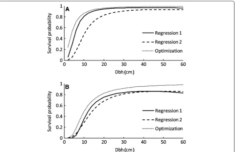
Figure 4One-year (A) and five-year (B) survival rates predicted by the fixed parts of mixed-effects models.

Table 4 Coefficients of fixed-effects diameter increment models

Predictor

Modelling approach

Constant –6.14591 –5.61685 0.88882

ln(d) 3.41191 2.31925 1.15958

d –0.15408 –0.05023 –0.08060

BAL –0.01522 –0.00569 –0.04803

√G –0.09034 –0.01232 –0.34133

Step – 0.07507 –

(7)

variable called dominance, calculated as DOMij= 1 – BALij/Gj, anduj~ N (0,σu) is random period factor.

In the‘Regression 2 approach’, the time interval between the measurement occasions was used as model predictor. The diameter increment model corresponding to this approach was:

idpij¼ expða0þa1ln dij þa2dij

þa3BALijþa4

ffiffiffiffiffi

Gj

p

þa5StepjþujÞ þeij

ð3Þ where idpij is the diameter increment of tree i during period j (cm) and Stepj is the length of the period (years). The corresponding survival model was:

Sij¼

1

1þexp b0þb1lndijþb2dþb3lnTj þb4DOMijþb5Stepjþuj

ð4Þ

In the optimization-based approach the diameter in-crement and mortality models were fitted simultaneously via nonlinear optimization (Nelder and Mead 1965), using diameter distributions as modelling data instead of tree-level growth and survival data (Pukkala et al. 2011). Starting from the initial diameter distribution of each Table 5 Coefficients of fixed-effects survival model

Predictor

Modelling approach

Constant 7.83597 6.36929 11.31540

ln(d) 1.54649 3.41518 2.94256

d _–0.02158 _–0.10010 _–0.07065

ln(T) _–3.14473 _–4.13006 _–5.06713

DOM 1.32723 1.41859 0.92033

Step _– _–0.21552 _–

d= diameter at breast height;T= stand age;DOM= dominance;Step= length of the projection period.

(8)

sample plot, the fitting procedure aims at reproducing the diameter distribution at the end of the measured growth interval by minimizing the sum of squared differ-ences between measured and predicted cumulative diameter distributions of tree frequency and stand basal area. The optimized decision variables were the coeffi-cients of the diameter increment and mortality models. Based on Pukkala et al. (2011), the objective function was defined as:

min zð Þ ¼θ X

K

k¼1

" XJk

j¼1

XIjk

i¼1

Gmjk dijk

−Gsjk dijk;θ

2

þ10−4X

Ijk

i¼1

Fmjk dijk

−Fsjk dijk;θ

2#

ð5Þ

where θ is the set of coefficients (a0,…a4, b0,…b4, and the period factors of the growth and survival models, see Equations 1 and 2) estimated as arg min z(θ), K is the number of plots,Jkis the number of periods of plotk,Ijk is the number of 3-cm diameter classes in period j of plot k, Gjkm(dijk) and Gjks(dijk) are, respectively, measured and simulated cumulative basal area (m2· ha–1) at diam-eter dijk (upper limit of diameter class i) at the end of period jof plot k, and Fjkm(dijk) and Fjks(dijk)are, respect-ively, measured and simulated cumulative number of trees per hectare at diameterdijk at the end of period j of plot k. The number of simultaneously estimated pa-rameters was 36 (2 × 13 period factors and 2 × 5 fixed re-gression coefficients).

All models were also fitted as fixed-effects models. The models were compared by simulating the stand de-velopment of each plot from the beginning to the end of each measurement interval. RSME (square root on the mean of squared errors) and bias were calculated for the ending basal area, ending number of living trees per hectare, and basal area increment. The‘Regression 2’ ap-proach was used both with 1-year time step and by pre-dicting the ending diameter and survival rate directly. When the time step was one year, the possible incom-plete year at the end of the growth period was simulated by adding a fraction of annual growth to the diameter (growth in 0.67 years was assumed to be 0.67 times an-nual growth). The survival rate of the incomplete year was obtained assStepwhere sis annual survival rate and

Stepis the length of the incomplete period in years.

Results and discussion

Diameter increment and survival models

The regression coefficients of the fixed predictors of mixed-effects diameter increment and survival models had the same signs in all three approaches (Tables 2 and 3).

BALand stand basal area decreased growth while tree size (dbh) had an increasing-decreasing effect. Increasing dom-inance improved survival and increasing age decreased it. Tree diameter improved survival, but the negative coeffi-cients of untransformed diameter indicate that survival will start to decrease again at large diameters.

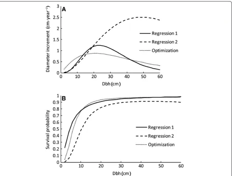
Visual inspection of the models revealed clear differences between modelling approaches (Figure 1). The‘Regression 1’approach predicts that diameter increment continues to increase with increasing tree diameter also in very large trees. However, this pattern could not be seen in the mod-elling data (Figure 2), suggesting that the fixed part of this mixed-effects model gives an erroneous picture on the growth pattern.

The obvious reason for the shape of ‘Regression 1’ model is that the random period factors also describe the influence of tree size. The assumption that the period fac-tors are independent and identically distributed was not met. This can be seen from Figure 3, which shows that the period factor of ‘Regression 1’model decreases with time. Decreasing period factor decreases the prediction for lar-ger diameters associated with later periods, implying that although the fixed part of the mixed-effects model seems unrealistic, the full model may predict realistic growths. This result verifies the conclusion that it may be unwise to use the fixed part of mixed-effects models in growth simu-lators (e.g., Temesgen et al. 2008; Garber et al. 2009; Pukkala et al. 2009; Shater et al. 2011; Groom et al. 2012; Heiðarsson and Pukkala 2012; de-Miguel et al. 2012; de-Miguel et al. 2013). As discussed by Burkhart and Tomé (2012) it would be better to refit the model without random parameters. Mixed-effects models can be used when the model is calibrated for a particular period.

Table 6 Statistics for full mixed-effects models (best in boldface,worst in italics)

Modelling and simulation approach

Regression 1 Regression 2 Regression 2 Optimization 1-year step 1-year step true step 1-year step Basal area

- bias (m2· ha–1) –1.09 1.43 1.10 –0.25

- RMSE (m2· ha–1) 4.28 3.99 4.20 2.27

Number of trees per hectare

- bias –27.07 –53.19 38.88 –0.42

- RMSE 100.23 137.98 128.16 35.19

Annual basal area increment

- bias (m2· ha–1) –0.297 0.709 0.151 0.005

- bias (%) 22.16 52.91 11.27 0.37

(9)

However, since calibration requires measurements from the same period, calibration cannot be done when one is predicting future growth.

The survival models are more similar to each other (Figure 4). In this case, the‘Regression 2’approach predicts lower annual survival rates than the other approaches (Figure 4 top). However, the differences between regression approaches 1 and 2 disappeared when survival rates were calculated for 5-year period (Figure 4 bottom). In this par-ticular case, the optimization-based model deviated slightly from the others.

Since it may not be recommendable to use non-calibrated mixed-effects models, i.e., their conditional predictions assuming that random parameters are zero,

all models were also fitted as fixed-effects model (Tables 4 and 5). The signs of the predictors again suggest similar growth and survival patterns in all models, but visual in-spection reveals that the‘Regression 2’model for diameter increment differs a lot from the other models (Figure 5). When the projection period is longer than one year, differ-ences in the shape of the relationship between diameter and diameter increment remain, but the magnitude of the difference is smaller for large trees (results not shown).

The fixed-effects survival models show similar patterns as the fixed parts of mixed-effects models (Figures 4 and 5). Also in this case the difference between ‘Regression 2’model and the other modes gets smaller for projection periods longer than one year.

(10)

Performance of the models

The models were used in simulation software to simulate the growth of all plots for each period. The mixed-effects models were used with and without period factors. The pre-dicted ending stand basal area and number of survivors were compared to their measured values. The RMSE (square root on the mean of squared errors) and bias were calculated also for the basal area increment of the period. Regression models fitted with the‘Regression 2’approach were used in two ways: by using one-year steps and by predicting the in-crement and survival of the whole period directly.

Of the full mixed-effects models, the optimization-based approach resulted in the best simulation results according to all criteria (Table 6, Figure 6). ‘Regression 2’approach used with the true length of the period (in-stead of simulating in 1-year steps) was the second best in predicting basal area increment and ending basal area. However, using ‘Regression 2’approach with 1-year time steps resulted in the lowest accuracy and precision.

As expected, the RMSEs and biases were larger (with some exceptions) when only the fixed parts of mixed models were used (Table 7). Ranking of the regression ap-proaches was now less straightforward. The optimization-based approach was the best according to all criteria.

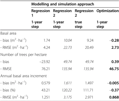
When the statistics were computed for the fixed-effects models,‘Regression 1’ approach turned out to be better than‘Regression 2’approach, and optimization was again clearly better than the other methods (Table 8). All regres-sion approaches resulted in very biased estimates of basal area increment.

Theoretically, full mixed-effects models should provide the most accurate and precise predictions. The second best should be fixed-effects models, and fixed parts of

mixed-effects models should be the worst (e.g., Temesgen et al. 2008; Garber et al. 2009; Pukkala et al. 2009; Shater et al. 2011; Heiðarsson and Pukkala 2012). Comparison of Tables 6, 7 and 8 reveals that this was not always the case. A probable reason for the deviations from expectations is that the statistics in Tables 6, 7 and 8 were computed for variables other than the response variables of regression analyses.

The best models were the full mixed-effects models re-covered by using the optimization-based approach. How-ever, period factors cannot be used when predicting future growth. Therefore, the models that should be used in sim-ulations are the fixed-effects models recovered with the optimization approach.

Supplementary models

Two supplementary models were developed for simulating the development of stand and tree height. Tree height may be a predictor in volume, taper and biomass equations and it is therefore useful to have models for height as well.

Of the tested dominant height models, the Hossfeld equation had good fitting statistics while being biologic-ally acceptable. Some other functions had slightly better fitting statistic but they gave unrealistic predictions out-side the range of variation of the modelling data. The se-lected dominant height model is:

H2¼ T

2 2

1:893þT2ðT1=H1−0:027T1−1:893=T1þ0:027T2Þ

ð6Þ

H refers to dominant height T to stand age. The de-gree of explained variance was 0.916 and the RMSE was Table 7 Statistics for the fixed parts of mixed-effects

models (best in boldface,worst in italics)

- bias (m2· ha–1) –1.07 3.01 3.82 0.18

- RMSE (m2· ha–1) 3.33 7.66 9.49 3.24

- bias –18.00 49.97 49.97 5.63

- RMSE 64.01 135.94 135.94 50.78

- bias (m2· ha–1) –0.885 0.355 0.463 0.013

- bias (%) 66.04 26.49 34.55 0.97

- RMSE (m2· ha–1) 1.322 1.339 1.476 0.976

Table 8 Statistics for the fixed-effects models (best in boldface,worst in italics)

- bias (m2· ha–1) 1.74 10.04 9.24 –0.28

- RMSE (m2· ha–1) 4.24 22.73 20.49 2.73

- bias –23.92 49.74 49.74 0.39

- RMSE 76.21 135.94 135.94 46.75

- bias (m2· ha–1) 0.579 1.611 1.497 –0.005

- bias (%) 43.21 120.22 111.71 –0.37

(11)

1.984 m. When the model is used to calculate site index,

T1 is replaced by measured stand age, H1by measured dominant height and T2by index age (30 years). When using the model to predict dominant height develop-ment,T1is replaced by index age,H1by site index, and

T2by the wanted projection age. Figure 7 shows that the model follows fairly well the measured sequences of dominant height in different plots.

The individual-tree height model is:

h¼1:3þðH−1:3Þ d D

0:201þ0:197 ln d

D ð Þ

ð7Þ

whereh is tree height (m),His dominant height (m), d is dbh (cm) andD is dominant diameter (cm). For this model, the degree of explained variance was 0.899 and the RMSE was 1.746 m. The model predicts that trees of a certain diameter are taller when the stand develops and its dominant height and dominant diameter increase (Figure8).

Conclusions

The study showed that regression models based on the assumption of linear growth or constant survival rate be-tween the measurement occasions, or using the length of measurement interval as a predictor, may lead to very biased predictions in growth simulations. Therefore, more sophisticated methods are needed to deal with irregular measurement intervals. The optimization method used in this study overcomes some of the problems related to other methods (Cao 2004; Nord-Larsen 2006). In addition, it

works also in cases where varying measurement interval is not the only shortcoming in the data (Pukkala et al. 2011, de-Miguel et al. 2014). The method can be used to calibrate an existing model or to fit a new model, or fit only a part of the models needed in simulation. For example, in the case that there are already models for diameter increment and survival, the method can be used to fit ingrowth models using data in which ingrowth trees cannot be separated from the other trees.

Earlier research has shown that the optimization-based modelling approach is competitive with individual-tree modelling based on regression analysis when there are no irregularities in the data (Pukkala et al. 2011; de-Miguel et al. 2014). This study showed that the method resulted

Figure 7Dominant height development in site indices 25, 30 and 35 m (dominant height at 30 years).The thin lines show the measured dominant height development of individual plots.

(12)

in clearly better models than obtained with more simplis-tic approaches to deal with irregular measurement inter-val. The benefit would of course be smaller if there was less variation in measurement interval.

The drawback of the method is poorer parameter iden-tifiability. The response variables of the models are not utilized in modelling, and the parameters of all models are estimated simultaneously. This may lead for instance to models that overestimate diameter growth, which is com-pensated for by underestimated survival rate. However, in-cluding both basal area and frequency distributions in the objective function decreases the likelihood of this kind of mutual cancellation of model errors. The problem may have been more serious if ingrowth model was esti-mated simultaneously with survival and diameter incre-ment model. In this case, overestimated ingrowth may be compensated for by overestimated mortality among the smallest diameter classes.

The optimization-based model recovery method used in this study makes a higher number of different types of observational plots available for individual-tree growth modelling. This saves money and time. There is no need to have the trees numbered or have a constant measure-ment interval. The method is not sensitive to errors in tree identification.

Competing interests

The authors declare that they have no competing interests.

Authors’contributions

MM provided the data. RJ, TP and SM conducted the analyses. All authors contributed to the writing of the manuscript. All authors read and approved the final manuscript.

Acknowledgements

We thank Kenya Forest Research Institute for support in data acquisition.

Author details

1_{University of Eastern Finland, PO Box 111, Joensuu 80101, Finland.}2_Kenya

Forest Research Institute, PO Box 20412, Nairobi 00200, Kenya.

Received: 17 April 2014 Accepted: 17 April 2014 Published: 28 August 2014

References

Bailey RL, Clutter JL (1974) Base-age invariant polymorphic site curves. For Sci 20:155–159

Burkhart HE, Tomé M (2012) Modelling Forest Trees and Stands. Springer Science + Business Media, Dordrecht, p 457

Cao QV (2000) Prediction of annual diameter growth and survival for individual trees from periodic measurements. For Sci 46:127–131

Cao QV (2004) Annual tree growth predictions from periodic measurements. In: Connor KF (ed) Proceedings of the 12thbiennial southern silvicultural research conference, Gen. Tech. Rep. SRS-71, USDA, Forest Service, Southern Research Station, Asheville, NC, pp 212–215

Cieszewski C, Bailey RL (2000) Generalized algebraic difference approach: a new methodology for derivation of biologically based dynamic site equations. For Sci 46:116–126

Clutter JL (1963) Compatible growth and yield models for loblolly pine. For Sci 9:354–371

Crecente-Campo F, Soares P, Tomé M, Diéguez-Aranda U (2010) Modelling annual individual-tree growth and mortality of Scots pine with data obtained

at irregular measurement intervals and containing missing observations. Forest Ecol Manage 260:1965–1974

de-Miguel S, Mehtätalo L, Shater Z, Kraid B, Pukkala T (2012) Evaluating marginal and conditional predictions of taper models in the absence of calibration data. Can J Forest Res 42(7):1383–1394

de-Miguel S, Guzmán G, Pukkala T (2013) A comparison of fixed- and mixed-effects modelling in tree growth and yield prediction of an indigenous neotropical species (Centrolobium tomentosum) in a plantation system. Forest Ecol Manage 291:249–258

de-Miguel S, Pukkala T, Morales M (2014) Using optimization to solve tree misidentification and uneven measurement interval problems in individual-tree modeling of Balsa stand dynamics. Ecol Eng 69:232–236 Diéguez-Aranda U, Burkhart HE, Rodriguez-Soalleiro R (2005) Modeling dominant

height growth of radiata pine (Pinus radiataD. Don) plantations in north-western Spain. Forest Ecol Manage 215:271–284

Diéguez-Aranda U, Burkhart HE, Amateis RL (2006) Dynamic site model for loblolly pine (Pinus taedaL.) plantations in the United States. For Sci 52(3):262_–272

Dvorak WS, Donahue JK (1992) CAMCORE cooperative research review 1980-1992. Department of Forestry. North Carolina State University, Raleigh, USA, p 93

Dvorak WS, Hodge GR, Kietzka JE, Malan F, Osorio LF, Stanger T (2000) Pinus patula. In: Conservation & Testing of Tropical & Subtropical Forest Tree Species by the CAMCORE Cooperative. College of Natural Resources, NCSU, Raleigh, NC. USA, pp 149–173

Garber SM, Temesgen H, Monleon VJ, Hann DW (2009) Effects of height imputation strategies on stand volume estimation. Can J Forest Res 39:681–690

Groom JD, Hann DW, Temesgen H (2012) Evaluation of mixed-effects models for predicting Douglas-fir mortality. Forest Ecol Manage 276:139–145 Heiðarsson L, Pukkala T (2012) Models for simulating the development of

Siberian larch (Larix sibiricaLedeb.) plantations in Hallormsstaður Iceland. Icel Agric Sci 25:13–23

Isango JA, Nshubemuki L (1998) Management of forest plantations in Tanzania with emphasis on planting and growth and yield. In: Pukkala T, Eerikäinen K (eds) Tree seedling production and management of plantation forests, vol 68, University of Joensuu, Faculty of Forestry, Research Notes., pp 25–38 Jaetzold R, Schmidt H (1983) Natural conditions and farm management. Farm

Management Handbook of Kenya, vol II C East Kenya. Ministry of Agriculture, Nairobi, Kenya

Lundqvist B (1957) On the height growth in cultivated stands of pine and spruce in Northern Sweden. Medddelanden Från Statens Skogforsk, Band 47(2):1_–64 Mabvurira D, Musokonyi C (1998) A review of plantation forestry in Zimbabwe.

In: Pukkala T, Eerikäinen K (eds) Tree seedling production and management of plantation forests, vol 68, University of Joensuu, Faculty of Forestry, Research Notes, pp 53–77

McDill ME, Amateis RL (1992) Measuring forest site quality using the parameters of a dimensionally compatible height growth function. For Sci 38:409–429 Muchiri GM, Muturi MN (1998) The state of forest plantations development,

management and future focus in Kenya. In: Pukkala T, Eerikäinen K (eds) Tree seedling production and management of plantation forests, vol 68, University of Joensuu, Faculty of Forestry, Research Notes., pp 11_–20 Nelder JA, Mead R (1965) A simplex method for function minimization. Comput J

7:308–313

Nord-Larsen T (2006) Modeling individual-tree growth from data with highly irregular measurement intervals. For Sci 52(2):198–208

Palmer ER, Gibbs JA (1974) Pulping qualities of plantation grownPinus patula

andPinus elliottiifrom Malawi, vol Report No. L37. Tropical Products Institute, London, UK, p 36

Peschel W (1938) Die mathematischen Methoden zur Herleitung der Wachstumsgesetze von Baum und Bestand und die Ergebnisse ihrer Anwendung. Tharandter Forstliches Jahrburch 89:169–247

Pukkala T, Lähde E, Laiho O (2009) Growth and yield models for uneven-sized forest stands in Finland. Forest Ecol Manage 258(3):207_–216

Pukkala T, Lähde E, Laiho O (2011) Using optimization for fitting individual-tree growth models for uneven-aged stands. Eur J For Res 130(5):829–839 Record SJ, Hess RW (1974) Timbers of the New World. Charles Lathrop Pack

Foundation, New Haven, USA, p 640

Richards FJ (1959) A flexible growth function for empirical use. J Exp Bot 10:290–300 Schumacher FX (1939) A new growth curve and its application to timber yield

(13)

Shater Z, de-Miguel S, Kraid B, Pukkala T, Palahí M (2011) A growth and yield model for even-agedPinus brutiaTen. stands in Syria. Ann For Sci 68(1)):149–157 Sloboda B (1971) Zur Darstellung von Wachstumprozessen mit Hilfe

von Differentialgleichungen erster Ordung. Mitteillungen der Badenwürttem-bergischen Forstlichen Versuchs und Forschungsanstalt, Freiburg

Stoffels A, van Soest J (1953) The main problems in sample plots. Ned Boschb Tijdschr 25:190–199

Temesgen H, Monleon VJ, Hann DW (2008) Analysis and comparison of nonlinear tree height prediction strategies for Douglas-fir forests. Can J Forest Res 38:553–565

Tomé M (1989) Modelação do crescimiento da árvore individual em povoamentos deEucalyptus globulusLabill. (1ª Rotação). Região Centro de Portugal. PhD thesis, ISA, Lisbon

Wormald TJ (1975) Pinus patula, Tropical Forestry Papers No. 7. Department of Forestry, Commonwealth Forestry Institute, University of Oxford., p 212 Wright JA (1994) Utilization ofPinus patula: An annotated bibliography. Oxford

Forestry Institute Occasional Papers, vol 45., p 73

doi:10.1186/s40663-014-0014-3

Cite this article as:Jumaet al.:Evaluation of different approaches to individual tree growth and survival modelling using data collected at irregular intervals–a case study forPinus patulain Kenya.Forest Ecosystems20141:14.