www.nat-hazards-earth-syst-sci.net/17/357/2017/ doi:10.5194/nhess-17-357-2017
© Author(s) 2017. CC Attribution 3.0 License.
Efficient bootstrap estimates for tail statistics
Øyvind Breivik1,2and Ole Johan Aarnes1
1Norwegian Meteorological Institute, Allegaten 70, 5007 Bergen, Norway 2Geophysical Institute, University of Bergen, Bergen, Norway
Correspondence to:Øyvind Breivik ([email protected]) Received: 6 July 2016 – Discussion started: 5 September 2016
Revised: 21 February 2017 – Accepted: 25 February 2017 – Published: 8 March 2017
Abstract.Bootstrap resamples can be used to investigate the tail of empirical distributions as well as return value esti-mates from the extremal behaviour of the sample. Specifi-cally, the confidence intervals on return value estimates or bounds on in-sample tail statistics can be obtained using bootstrap techniques. However, non-parametric bootstrap-ping from the entire sample is expensive. It is shown here that it suffices to bootstrap from a small subset consisting of the highest entries in the sequence to make estimates that are es-sentially identical to bootstraps from the entire sample. Simi-larly, bootstrap estimates of confidence intervals of threshold return estimates are found to be well approximated by using a subset consisting of the highest entries. This has practical consequences in fields such as meteorology, oceanography and hydrology where return values are calculated from very large gridded model integrations spanning decades at high temporal resolution or from large ensembles of independent and identically distributed model fields. In such cases the computational savings are substantial.
1 Introduction
Bootstrap resamples of time series are commonly used to ob-tain non-parametric confidence intervals (CIs) on return val-ues (Naess and Clausen, 2001; Naess and Hungnes, 2002) and to investigate the behaviour of the tail of the empirical distribution (Coles, 2001; Beirlant et al., 2006; Qi, 2008). Although non-parametric CIs tend to be too narrow, see Ky-selý (2008), the procedure itself is algorithmically and nu-merically straightforward to implement and is thus a conve-nient technique for rapidly assessing the width of CIs with-out having to assume a certain parametric distribution. How-ever, this approach quickly becomes cumbersome for large
data sets as it demands random draws from the entire sam-ple which subsequently must be sorted to get to the upper percentiles. When handling long model integrations in mete-orology, hydrology and oceanography with spatially gridded fields of typically 106grid points this brute-force approach becomes impractical. Such quantities are regularly encoun-tered when estimating return levels from atmospheric reanal-yses (Kalnay et al., 1996; Saha et al., 2010; Compo et al., 2011; Dee et al., 2011; Poli et al., 2016), wave hindcasts (Swail and Cox, 2000; Caires and Sterl, 2005; Gaslikova and Weisse, 2006; Breivik et al., 2009; Reistad et al., 2011; Aarnes et al., 2012) and long climate integrations that cover decades or even centuries (Hersbach et al., 2015). When even larger data sets are used, such as the ensembles of seasonal integrations (Stockdale et al., 2011; Molteni et al., 2011), as was done by Van den Brink et al. (2005) on a sample amount-ing to nearly 1000 years, findamount-ing ways to reduce the size of the samples becomes essential. That is the subject of this pa-per.
We will present a simple argument for why it is sufficient to retain only a small subsetK0consisting of the highest en-tries in a sample when estimating tail statistics such as return levels and their associated CIs by means of non-parametric bootstrapping. These highest entries will normally only rep-resent a small fraction of the total sample. This reduces the need for sorting and storage by several orders of magnitude. The method also reduces the task of sorting the original sam-ple as only theK0highest entries are kept.
the method laid out in Sect. 2 can be used in practice to de-termine how many entries must be kept in order to perform an unbiased bootstrap. Section 4 summarizes the results and presents the conclusions.
2 Bootstrapping from theK0highest entries in a sample
Consider the sample D0 of independent and identi-cally distributed (iid) random numbers X1, X2, . . ., XN. Let XN,1≤XN,2≤ · · · ≤XN,N denote the order statis-tics on D0. When investigating a statistic θ which is a function of the k highest entries in D0, i.e. θ=
f (XN,N−k+1, XN,N−k+2, . . ., XN,N), it is common to form
M bootstrap resamples D1,D2, . . .,DM, each of length N (Diaconis and Efron, 1983; Efron and Gong, 1983). This method can be used to compute the CIs around extreme value estimates (Breivik et al., 2013, 2014). The proce-dure is computationally intensive and memory consuming, as it involves bootstrapping and storing M×N numbers and performing M sorts, each a process of O(Nlog2N )
operations (Press et al., 2007, pp. 423–427). Since we are only interested in combinations of the k highest en-tries in the resamples D1,D2, . . .,DM, we will explore the possibility of instead resampling from only the high-est XN,N−K0+1, XN,N−K0+2, . . ., XN,N−k+1, . . ., XN,N en-tries inD0(K0> k). This will be referred to as the resample threshold and is sometimes more conveniently written as the percentage of data left out,P0=100(1−K0/N ).
The probability of drawing one of the highestK0entries in
D0is a binomial problem with probabilityp=K0/N. The probability of making exactly k draws (with replacement) from the highestK0inN draws is thus given by the bino-mial probability mass function (Zwillinger, 1996, p. 581)
fbinom(k;N, p)=P (X=k)= N
k
pk(1−p)N−k, (1) where X is a random variable representing the number of draws. The probability of drawing fewer than the requiredk
entries from the highestK0is given by the binomial cumula-tive distribution function
Fbinom(k−1;N, p)=P (X < k)= k−1 X
i=0 N
i
pi(1−p)N−i. (2)
A full bootstrap resample Di of length N from D0 will contain Ki entries from the highest K0, and Ki∼ Binom(N, p)whereE[Ki] =K0since the expected (mean) value of the binomial distribution (Eq. 1) is
µbinom=Np=K0. (3)
The variance is
σbinom2 =Np(1−p)=K0−K02/N≈K0 when K0N.
(4) Denote a short bootstrap resample from theK0highest en-tries inD0asDei. Two conditions must be met forDei to be an unbiased substitute forDi:
1. The numberK0must be set large enough that the prob-ability that we miss entries smaller thanXN,N−K0+1in D0is below a chosen thresholdpc.
2. The lengthKeiofDeimust have the same mean and vari-ance asKi(Eqs. 3–4).
To fulfil condition (1) it is sufficient to decide on an accept-able level forpc. This probability can be found by consulting Eq. (2). It is important to note that choosingK0too small will bias the statisticeθ=f (Dei)since it will be estimated from bootstrap samples that miss entries smaller thanXN,N−K0+1. We will for this reason refer topcas the probability of con-tamination as it gives the probability that the bootstrap es-timate is biased because we have kept too few entries from the original sampleD0. A very conservative bound onp, and thus onK0=Np, can be found quickly by consulting Ho-effding’s formula (Hoeffding, 1963),
F (k;N, p)≤exp
−2(Np−k) 2
N
, (5)
valid whenk≤Np. A useful quantity is the ratior=K0/ k of upper entries retained (K0) and the minimum number k required to form a bootstrap estimate of the statistic in ques-tion for a given probability of contaminaques-tionpc. This can be found from Eq. (2), but whenN is large the Poisson distri-bution is a good approximation and more practical to work with,
FPoisson(k−1;rk)=P (X < k)=e−rk k−1 X
i=0
(rk)i
i! . (6)
Figure 1 shows the minimum acceptable ratioK0/ kas a function ofkfor levels ofpcranging from 10−5to 0.05. The probabilities can be computed from Eq. (2) (or more conve-niently from Eq. 6). As can be seen, for all values ofk, the ratio is comfortably below 15, and for values ofklarger than 10 a ratio of 3 is sufficient even for a confidence level of 10−5. See the Appendix for a more detailed explanation of the ratio curves used throughout.
Condition (2) can be handled by randomly perturbing the size of the resamples,Kei, such that it mimics the number of draws,Ki ∼Binom(N, p), that would have been made from the upperK0entries ofD0in a full bootstrapDi. In practice, as we shall see, the statistics are quite insensitive to these per-turbations as long asK0has been chosen sufficiently large.
3 Bootstrapping confidence intervals
100 101 102 103 104 105
k
1 2 3 4 5 6 7 8 9 10 11 12 13
r
=
K0
/k
0.05 Probability of contamination pc 0.01
0.005 0.001 0.0005 0.0001 1e-05
Figure 1.The ratioK0/ kas a function ofk, the minimum number of bootstrapped entries needed for the statistic in question, for lev-els of probability of contamination ranging from 10−5(uppermost curve) to 0.05 (lowermost curve). The curve representing 1 % prob-ability of contamination is marked in red (with diamonds) as it is a reasonable confidence level.
0 2 4 6 8 10 12 14 16
Significant wave height, Hs [m]
0 5000 10000 15000 20000 25000 30000 35000
P99.1P99.7
Ekofisk, all +240-h ensemble forecasts
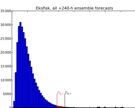
Figure 2.Histogram of the significant wave height from archived ensemble forecasts in the central North Sea (Ekofisk, 56.5◦N, 003.2◦E) at+240 h lead time. Entries aboveP99.1, corresponding to thresholdU0, are coloured red whilst entries exceedingP99.7, corresponding to the upper threshold,u, are in black. The highest entries are individually marked with asterisks.
tail statistics for a data set of independent ensemble forecasts at long lead time (N=330 000). We use archived ensemble forecasts (Molteni et al., 1996) of significant wave height in the central North Sea (near the Ekofisk oil field at 56.5◦N, 003.2◦E; a histogram of the data set used is shown in Fig. 2) at a forecast lead time of 240 h. One-hundred-year return val-ues from these ensembles have previously been reported by Breivik et al. (2013, 2014).
3.1 Example 1: confidence intervals on in-sample return estimates
Consider as an example the problem of how to calculate in-sample return estimates from the in-sample of independent fore-casts presented above. These forefore-casts can be considered iid (as they are not from correlated time series). An in-sample return estimate is calculated directly from the tail of the em-pirical distribution rather than by applying extreme value analysis. As explained by Breivik et al. (2013) the indepen-dent forecasts presented in Fig. 2 add up to the equivalent of 229 years under the assumption that each forecast repre-sents a time interval1t=6 h. A 100-year return estimate is then a linear interpolation betweenXN,N−1andXN,N−2(the second and third highest entries inD0),
H100=0.67XN,N−1+0.33XN,N−2. (7) Now, clearlyk=3 since we need the second and third high-est entries in our resamples to form a return high-estimate. Let us now tentatively keep theK0=1000 highest entries and bootstrap from these instead of from the entire sequence to compute the CIs on the linear combination of the second and third highest entries given by Eq. (7). The sizeKei of the resamples,Dei, is drawn from the binomial distribution (Eqs. 3–4) withµ=K0andσ2≈K0. What is the probabil-itypcthat one of the three highest entries in a bootstrapped sequence should not have come from the 1000 highest entries that we have retained (i.e. should depend on entries contained in the bulk of the sample that we discarded)? It is clear that the probability of drawing one of the highest 1000 entries is
p=1000/330 000, and from Eq. (2) we find that the prob-ability of picking too few (<3) entries from theK0highest is
F (2;330 000, p)=P (X≤2)= 2 X
i=0
330 000 i
pi(1−p)330 000−i, (8) which is indistinguishable from zero to double precision. Re-ducing the numberK0 to 10 (r≈3) raises the probability of contaminating the resamples by entries from the lower
N−K0 to 0.002. This can also be confirmed by consult-ing Fig. 1 for the combinationk=3, r=3. ForM=1000 resamples we may thus expect on average two resamples to be contaminated by values from the lowerN−K0values in the original sequence. A very safe compromise in this case is
K0=100 (r≈33). Consulting Fig. 1 shows that fork=3,
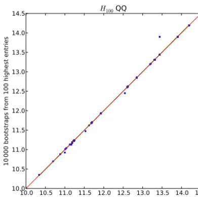
r=33 we are well below a probability of contamination of 10−5. The quantile–quantile (QQ) plot in Fig. 3 shows that resampled return estimates of significant wave height from the full sampleD0(see Fig. 2) have practically the same dis-tribution as resamples from the upperK0=100 entries.
10.0 10.5 11.0 11.5 12.0 12.5 13.0 13.5 14.0 14.5 10000 bootstraps 10.0 10.5 11.0 11.5 12.0 12.5 13.0 13.5 14.0 14.5 10 00 0 bo ot str ap s f ro m 1 00 h igh es t e nt rie s
H100
Figure 3.A quantile–quantile comparison of 10 000 bootstrapped direct 100-year return estimates of significant wave height taken from a forecast ensemble (Breivik et al., 2013) versus a bootstrap from the upper 100 entries in the sample. The 45◦line is shown in red.
10.0 10.5 11.0 11.5 12.0 12.5 13.0 13.5 14.0 14.5 10000 perturbed-length bootstraps from 100 highest entries 10.0 10.5 11.0 11.5 12.0 12.5 13.0 13.5 14.0 14.5 10 00 0 un pe rtu rb ed b oo tst ra ps fr om 1 00 h igh es t e nt rie
s H100
Figure 4. A quantile–quantile (QQ) comparison of M=10 000
bootstraps De1,De2, . . .,DeM of variable length Ke1,Ke2, . . .,KeM against bootstraps of fixed lengthK0, all from the upper 100 en-tries in the original sequenceD0. The difference is very small.
turns out to be rather insignificant as long as K0 is cho-sen sufficiently large. This is demonstrated in the QQ plot in Fig. 4 where we see that perturbed-length estimates (ab-scissa) closely match the distribution of fixed-length esti-mates (ordinate). However, choosingK0too small will bias the statistic in question. This is illustrated in Fig. 5 where we see that bootstrap estimates from too-short subsets of the original sample (K0 chosen too small) are biased high. As
K0 approaches 30 (r=10), the mean and standard
devia-tion of the return estimates approach their asymptotic values. These findings are in accordance with what we find by con-sulting Fig. 1 where we see thatk=3, r=10 has a prob-ability of contaminationpc less than 10−5. It is also of in-terest to investigate just how many bootstrap resamples are actually needed to obtain CIs from a non-parametric boot-strap technique. In Fig. 5 we choseM=10 000. As Fig. 6 shows, this is clearly excessive for reasonable thresholdsK0. In fact, Efron and Tibshirani (1993) state that 200 resamples are normally enough. We find this to be on the low side in our case, as Fig. 6 shows. However, 1000 resamples is suffi-cient in this case, but this should be investigated in each case. Breivik et al. (2014) found (see their Supplementary Fig. 7) that for a similar data set, 500 resamples would be sufficient when employing a generalized Pareto distribution (GPD) on threshold exceedances.
3.2 Example 2: confidence intervals on upper percentiles
A similar problem to the estimation of CIs for in-sample return values is how to obtain the CI for the highest per-centiles, e.g. the 99th percentile (P99). The upper percentile is frequently used when investigating trends in for example the wind and wave height climate (see e.g. Wang and Swail (2001, 2002)). In order to construct a bootstrap estimate of
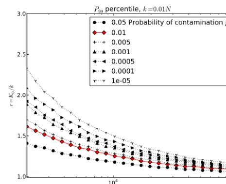
P99 brute force it is necessary to resample the entire sam-ple D0 and sort the bootstrap to get to the N/100th high-est entry. However, Fig. 1 tells us that whenk=N/100 is large (as it will be whenN is large), we can with extremely high certainty say that keeping theK0=2k highest entries is enough to perform a bootstrap resample exercise for the CI onP99. In fact,K0=1.2kis sufficient for all significance levels plotted in Fig. 1. This means that in order to obtain a CI forP99we need only find the entryXN,N−kthat corresponds toP99from the original sampleD0and retain entries higher thanXN,N−1.2k. Figure 7 shows how the ratior decreases as the sample sizeN increases. It is clear that for all prob-abilities of contamination investigated, a ratio ofK0/ k=2 is sufficient whenNis larger than 2000. Obviously, samples smaller thanO(103)do not pose computationally demanding problems anyway and are of no interest to us in this context. Figure 8 illustrates for a fixed probability of contamination
pc=0.01 that even as we go to higher percentiles (the up-permost curve showsP99.9), a ratioK0/ k=2 is sufficient as the sample sizeN exceeds 104(see the Appendix for more details on the ratio curves).
3.3 Example 3: confidence intervals on return estimates from threshold exceedances
han-99.94 99.95 99.96 99.97 99.98 99.99
Resample threshold, 100(1−K / N0 ), N= 330 000
11.5 12.0 12.5 13.0 13.5 14.0
Significant wave height [m]
Mean SD
5 12 25 50 100
200 K0
Figure 5.Mean and standard deviation on 100-year in-sample re-turn estimates based onM=10 000 bootstrap resamples for various choices of resample thresholdK0for the sample in Fig. 2. A min-imum ofk=3 entries are required to form the return estimate (see Eq. 7). For choices ofK0smaller than 30 (corresponding to a ratio
r=K0/ k=10) the bootstrap resamples are biased high.
0 2000 4000 6000 8000 10000
Number of bootstrap resamples, M
11.0 11.5 12.0 12.5 13.0 13.5 14.0
Significant wave height [m]
In-sample 100-year return level estimates
Mean SD
Figure 6.Mean and standard deviation on 100-year in-sample re-turn estimates with a thresholdK0=1000 as a function of number of bootstrap resamples,M. ForM >1000 the CIs are quite stable.
dled to estimate return levels (Coles, 2001). GPD gives the relevant extreme value distribution for independent ex-ceedances above a thresholdu(Coles, 2001, 75–77),
H (y)=1−
1+ξy eσ
−1/ξ
. (9)
Here y=Xi−u,y >0 are exceedances above a threshold
u=XN,N−k+1(remember thatXN,N−k+1is thekth highest entry in the sampleD0) andeσ is a scale parameter which is a function of the thresholdu, andξ is the shape parameter.
104 105
N
1.0 1.5 2.0 2.5 3.0
r
=
K0
/k
P99
percentile,
k=0.01N0.05 Probability of contamination
pc0.01
0.005
0.001
0.0005
0.0001
1e-05
Figure 7.Bootstrapping the 99th percentile, P99. The ratio r=
K0/ kis shown as a function of sample size N. Here, the mini-mum number of entries required is simply the upper 1 % (P99), so
k=N/100. Various levels of probability of contaminationpc are shown, and for sample sizes larger than approximately 2000, a ra-tior=2 is sufficient. The curve representing 1 % probability of contamination is marked in red (with diamonds) as it represents a reasonable confidence level.
A brute-force approach would be to makeN draws from
D0 (with replacement) and repeat this procedure M times. Then, GPD return estimates would be computed for each of the resulting bootstrap sequences D1,D2, . . .,DM. Say we want to try to instead retain only theK0 entries exceeding a threshold U0, where U0< u, corresponding to the entry
XN,N−K0+1in the original sampleD0. From these we need to draw at leastkentries, from which we will make return estimates. The question is again how many entries (K0) must be kept to arrive at an acceptably low probabilitypcthat the statistic should really be based on entries below the threshold
U0.
confi-104 105
N
1.0 1.5 2.0 2.5 3.0 3.5 4.0 4.5 5.0
r
=
K0
/k
Probability of contamination pc=0.01
0.9 Percentile P, k=(1−P)N/100
0.95 0.97 0.99 0.999
Figure 8. Bootstrapping the upper percentiles P=
P90, P95, P97, P99 and P99.9. The ratio r=K0/ k is shown as a function of sample size N. Here, the minimum number of entries required is k=(1−P )N/100. The probability of con-tamination is kept fixed atpc=0.01. At sample sizes larger than approximately 104, a ratio r=2 is sufficient for all percentiles investigated. The curve representing the 99th percentile is marked in red (with diamonds) and corresponds to the red curve in Fig. 7.
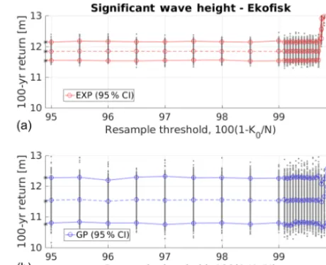
dence interval and the mean return value based onM=1000 bootstrap resamples for various choices of resample thresh-old 100(1−K0/N )(i.e. the percentage of data omitted) are practically identical to the CIs based onD0(marked as as-terisks). Only when r=K0/ k comes close to unity do we experience fluctuations and biases (i.e. the resample thresh-old nearly coincides with the number of tail entries required to form a return estimate, in this case the thresholdP99.7).
4 Conclusions
CIs and other statistics of the extremes and the tail of empir-ical distributions are commonly found using non-parametric bootstrap techniques. Here we have shown that it is unnec-essary to bootstrap from the entire original sample. The ac-tual number K0 highest entries that must be kept to make unbiased bootstrap estimates for the tail of an empirical dis-tribution depends on K0=Npas well as on the numberk highest entries that are required for the statistic in question. The examples in the previous sections calculatedpcgiven a predetermined numberK0of tail entries that have been kept. This is a realistic approach as in practice we often retain a larger part of the tail of an empirical distribution than what is strictly needed since the same data set is used to compute other statistics. It is then sufficient to consult Eq. (2) to de-termine whetherK0is sufficiently large. A quick estimate of the probability of contamination can be made by consulting Fig. 1.
Figure 9.The upper and lower 95 % CIs and the mean 100-year re-turn estimates (dashed) based onM=1000 bootstrap resamples for various choices of resample thresholdK0for the sample in Fig. 2. Upper panel: a GPD with shape parameterξ=0 (exponential distri-bution). Lower panel: a GPD with freely varying shape parameter. Individual bootstrap estimates are marked in grey. Estimates based on the full sampleD0are marked as asterisks on the ordinate.
The advantages of restricting resamples to a small subset
K0consisting of the highest entries inD0can be summarized as follows. First, only the upperK0entries need be kept and sorted in the original data set. This offers substantial sav-ings in cases like those described by Breivik et al. (2013, 2014) where a very large number of forecasts (>300 000) are handled, each consisting of more than 60 000 grid points in space. Second, the size of the resamples is also reduced fromN to an average sizeK0, whereK0is usually a very small fraction ofN, typically less than 1 %. Third, this re-duction in resample size also means that the cost of sorting the resamples to get to the highest entries is greatly reduced, as the problem is now linear in the number of bootstrap re-samplesMsince each sort isO(K0log2K0), which is now a constant number independent of the size of the original sam-ple (or a small fraction of it, as in the 99th percentile shown in Example 2).
called for. In particular, the test inversion bootstrap (Carpen-ter, 1999) is a promising method where the test inversion refers to the duality between hypothesis testing and confi-dence intervals. Schendel and Thongwichian (2015, 2017) show how this method, originally developed for estimation of statistics of single parameters in the presence of nuisance parameters, can be extended to handle return levels which depend on three parameters for both the generalized extreme value distribution and GPD by utilizing a maximum likeli-hood technique. However, non-parametric bootstraps repre-sent a quick and hypothesis-free approach to obtaining CIs, and as the results presented show we can comfortably as-sume that the results will remain unchanged if we select a small subset of the original sample, provided we follow the procedure outlined in Sect. 2.
Appendix A: Consulting the ratio curves
The ratio curves presented in Figs 1, 7 and 8 are conve-nient for quickly establishing how many entries (K0) must be kept in order to form an unbiased resample that depends on the highestkentries. The relationship between Fig. 1 and Fig. 7 can be illustrated as follows. If we assume N large we can use Fig. 1. In practice we can chooseN=2×10³ without violating the assumption that N is large. Now as-sume that the statistic in question is the 99th percentile, i.e.
k=N/100=20. Let us choose a probability of contamina-tionpc=0.01 (this corresponds to the red curve marked with diamonds in Fig. 1). We find the ratio to be 1.6, i.e. we will need to keep 60 % more entries than the entry corresponding toP99. The corresponding curve in Fig. 7 is also marked in red. Here, the location on thexaxis to read off isN=2×10³, which lies on the y axis, and the ratio is again found to be 1.6. A more realistic example in terms of sample size would beN=105(andk=N/100=103). Now we find from ei-ther Fig. 1 or Fig. 7 that with a probability of contamination
Competing interests. The authors declare that they have no conflict of interest.
Acknowledgements. This study was carried out with support from the Research Council of Norway through the ExWaCli project (grant no. 226239) and the follow-up, ExWaMar (grant no. 256466).
Edited by: N. Pinardi
Reviewed by: S. Caires and R. Katz
References
Aarnes, O. J., Breivik, Ø., and Reistad, M.: Wave Ex-tremes in the Northeast Atlantic, J. Climate, 25, 1529–1543, doi:10.1175/JCLI-D-11-00132.1, 2012.
Beirlant, J., Goegebeur, Y., Segers, J., and Teugels, J.: Statistics of extremes: theory and applications, John Wiley & Sons, 99–123, 2006.
Breivik, Ø., Gusdal, Y., Furevik, B. R., Aarnes, O. J., and Reis-tad, M.: Nearshore wave forecasting and hindcasting by dynam-ical and statistdynam-ical downscaling, J. Marine Syst., 78, S235–S243, 2009.
Breivik, Ø., Aarnes, O. J., Bidlot, J.-R., Carrasco, A., and Saetra, Ø.: Wave Extremes in the Northeast Atlantic from Ensemble Fore-casts, J. Climate, 26, 7525–7540, 2013.
Breivik, Ø., Aarnes, O., Abadalla, S., Bidlot, J.-R., and Janssen, P.: Wind and Wave Extremes over the World Oceans From Very Large Ensembles, Geophys. Res. Lett., 41, 5122–5131, doi:10.1002/2014GL060997, 2014.
Caires, S. and Sterl, A.: A new nonparametric method to cor-rect model data: application to significant wave height from the ERA-40 re-analysis, J. Atmos. Ocean. Tech., 22, 443–459, doi:10.1175/JTECH1707.1, 2005.
Carpenter, J.: Test inversion bootstrap confidence intervals, J. R. Stat. Soc. B, 61, 159–172, doi:10.1111/1467-9868.00169, 1999. Coles, S.: An introduction to statistical modeling of extreme values,
Springer Verlag, 78–84, 2001.
Compo, G. P., Whitaker, J. S., Sardeshmukh, P. D., Matsui, N., Al-lan, R. J., Yin, X., Gleason, B. E., Vose, R. S., Rutledge, G., Bessemoulin, P., Brönnimann, S., Brunet, M., Crouthamel, R. I., Grant, A. N., Groisman, P. Y., Jones, P. D., Kruk, M. C., Kruger, A. C., Marshall, G. J., Maugeri, M., Mok, H. Y., Nordli, Ø., Ross, T. F., Trigo, R. M., Wang, X. L., Woodruff, S. D., and Worley, S. J.: The Twentieth Century Reanalysis Project, Q. J. Roy. Me-teor. Soc., 137, 1–28, doi:10.1002/qj.776, 2011.
Dee, D. P., Uppala, S. M., Simmons, A. J., Berrisford, P., Poli, P., Kobayashi, S., Andrae, U., Balmaseda, M. A., Balsamo, G., Bauer, P., Bechtold, P., Beljaars, A. C. M., van de Berg, L., Bid-lot, J., Bormann, N., Delsol, C., Dragani, R., Fuentes, M., Geer, A. J., Haimberger, L., Healy, S. B., Hersbach, H., Hólm, E. V., Isaksen, L., Kållberg, P., Köhler, M., Matricardi, M., McNally, A. P., Monge-Sanz, B. M., Morcrette, J.-J., Park, B.-K., Peubey, C., de Rosnay, P., Tavolato, C., Thépaut, J.-N., and Vitart, F.: The ERA-Interim reanalysis: Configuration and performance of the data assimilation system, Q. J. Roy. Meteor. Soc., 137, 553–597, doi:10.1002/qj.828, 2011.
Diaconis, P. and Efron, B.: Computer intensive methods in statistics, Sci. Am., 248, 116–130, 1983.
Efron, B. and Gong, G.: A Leisurely Look at the Bootstrap, the Jackknife, and Cross-Validation, Am. Stat., 37, 36–48, 1983. Efron, B. and Tibshirani, R. J.: An introduction to the bootstrap,
CRC press, p. 50, 1993.
Gaslikova, L. and Weisse, R.: Estimating near-shore wave statistics from regional hindcasts using downscaling techniques, Ocean Dynam., 56, 26–35, 2006.
Hersbach, H., Peubey, C., Simmons, A., Berrisford, P., Poli, P., and Dee, D.: ERA-20CM: a twentieth-century atmospheric model ensemble, Q. J. Roy. Meteor. Soc., 141, 2350–2375, doi:10.1002/qj.2528, 2015.
Hoeffding, W.: Probability inequalities for sums of bounded random variables, J. Am. Stat. Assoc., 58, 13–30, doi:10.1080/01621459.1963.10500830, 1963.
Kalnay, E., Kanamitsu, M., Kistler, R., Collins, W., Deaven, D., Gandin, L., Iredell, M., Saha, S., White, G., Woollen, J., Zhu, Y., Leetmaa, A., Reynolds, R., Chelliah, M., Ebisuzaki, W., Higgins, W., Janowiak, J., Mo, K. C., Ropelewski, C., Wang, J., Jenne, R., and Joseph, D.: The NCEP/NCAR 40-Year Reanalysis Project, B. Am. Meteorol. Soc., 77, 437–472, 1996.
Kyselý, J.: A Cautionary Note on the Use of Nonpara-metric Bootstrap for Estimating Uncertainties in Extreme-Value Models, J. Appl. Meteorol. Clim., 47, 3236–3251, doi:10.1175/2008JAMC1763.1, 2008.
Molteni, F., Buizza, R., Palmer, T. N., and Petroliagis, T.: The ECMWF ensemble prediction system: methodology and validation, Q. J. Roy. Meteor. Soc., 122, 73–119, doi:10.1002/qj.49712252905, 1996.
Molteni, F., Stockdale, T., Balmaseda, M. A., Balsamo, G., Buizza, R., Ferranti, L., Magnusson, L., Mogensen, K., Palmer, T. N., and Vitart, F.: The new ECMWF seasonal forecast system (System 4), ECMWF Technical Memorandum 656, European Centre for Medium-Range Weather Forecasts, 2011.
Naess, A. and Clausen, P.: Combination of the Peaks-over-treshold and bootstrapping methods for extreme value prediction, Struct. Saf., 23, 315–330, 2001.
Naess, A. and Hungnes, B.: Estimating Confidence Intervals of Long Return Period Design Values by Bootstrapping, J. Offshore Mech. Arct., 124, 2–5, doi:10.1115/1.1446078, 2002.
Poli, P., Hersbach, H., Dee, D., Berrisford, P., Simmons, A., Vitart, F., Laloyaux, P., Tan, D., Peubey, C., Thepaut, J.-N., Trémolet, Y., Hólm, E., Bonavita, M., Isaksen, L., and Fisher, M.: ERA-20C: An Atmospheric Reanalysis of the Twentieth Century, J. Climate, 29, 4083–4097, doi:10.1175/JCLI-D-15-0556.1, 2016. Press, W. H., Teukolsky, S. A., Vetterling, W. T., and Flannery, B. P.:
Numerical Recipes in C, 3rd Edn., Cambridge University Press, Cambridge, 2007.
Qi, Y.: Bootstrap and empirical likelihood methods in extremes, Ex-tremes, 11, 81–97, doi:10.1007/s10687-007-0049-8, 2008. Reistad, M., Breivik, Ø., Haakenstad, H., Aarnes, O. J., Furevik,
B. R., and Bidlot, J.-R.: A high-resolution hindcast of wind and waves for the North Sea, the Norwegian Sea, and the Barents Sea, J. Geophys. Res., 116, C05019, doi:10.1029/2010JC006402, 2011.
H.-Y., Juang, H.-M. H., Sela, J., Iredell, M., Treadon, R., Kleist, D., Van Delst, P., Keyser, D., Derber, J., Ek, M., Meng, J., Wei, H., Yang, R., Lord, S., Van Den Dool, H., Kumar, A., Wang, W., Long, C., Chelliah, M., Xue, Y., Huang, B., Schemm, J.-K., Ebisuzaki, W., Lin, R., Xie, P., Chen, M., Zhou, S., Higgins, W., Zou, C.-Z., Liu, Q., Chen, Y., Han, Y., Cucurull, L., Reynolds, R. W., Rutledge, G., and Goldberg, M.: The NCEP climate fore-cast system reanalysis, B. Am. Meteorol. Soc., 91, 1015–1057, doi:10.1175/2010Bams3001.1, 2010.
Schendel, T. and Thongwichian, R.: Flood frequency analysis: Con-fidence interval estimation by test inversion bootstrapping, Adv. Water Resour., 83, 1–9, doi:10.1016/j.advwatres.2015.05.004, 2015.
Schendel, T. and Thongwichian, R.: Confidence intervals for re-turn levels for the peaks-over-threshold approach, Adv. Water Resour., 99, 53–59, doi:10.1016/j.advwatres.2016.11.011, 2017. Stockdale, T., Anderson, D., Balmaseda, M., Doblas-Reyes, F., Ferranti, L., Mogensen, K., Palmer, T., Molteni, F., and Vi-tart, F.: ECMWF seasonal forecast system 3 and its predic-tion of sea surface temperature, Clim. Dynam., 37, 455–471, doi:10.1007/s00382-010-0947-3, 2011.
Swail, V. R. and Cox, A. T.: On the use of NCEP-NCAR reanalysis surface marine wind fields for a long-term North Atlantic wave hindcast, J. Atmos. Ocean Tech., 17, 532–545, 2000.
Van den Brink, H., Können, G., Opsteegh, J., Van Oldenborgh, G., and Burgers, G.: Estimating return periods of extreme events from ECMWF seasonal forecast ensembles, Int. J. Climatol., 25, 1345–1354, doi:10.1002/joc.1155, 2005.
Wang, X. and Swail, V.: Changes of extreme wave heights in Northern Hemisphere oceans and related atmospheric circulation regimes, J. Climate, 14, 2204–2221, 2001.
Wang, X. and Swail, V.: Trends of Atlantic wave extremes as sim-ulated in a 40-yr wave hindcast using kinematically reanalyzed wind fields, J. Climate, 15, 1020–1035, 2002.