Multi-Objective Method For Electrical Distribution Network Using Modified Firefly Algorithm

281 _____________________

 Ali Mahmudi, Hamid Keyvani

Department of Electrical Engineering, Kazerun Branch, Islamic Azad University, Kazerun, Iran Email:[email protected]

Multi-Objective Method For Electrical Distribution

Network Using Modified Firefly Algorithm

Ali Mahmudi, Hamid Keyvani

Abstract: Due to the increasing consumption of electrical energy, appropriate design of future network and reconfiguration of the current network is of considerable importance. In this paper, the proposed method based on stochastic load flow in the presence of a wind turbine as well as the modified firefly optimization algorithm has been reviewed for optimal management of reconfiguration strategy and the IEEE 32-bus standard network has been used to observe its performance. The objective functions evaluated include: 1) minimization of the total cost of active power losses in the network, 2) reducing the total network operating costs and 3) reducing total emissions produced by the network. The appropriate solution of reconfiguration problem is also considered regarding the uncertainty caused by the wind turbines.

Index Terms: Multi-objective optimization, load flow, reconfiguration, wind turbine, distribution system, uncertainty.

————————————————————

1. Introduction

Electric power distribution networks due to advantages such as less short-circuit current and easier coordination of protection systems, in most cases are designed and operated in a radial form. On the other hand, this would reduce the reliability of the subscribers, and in some cases increase power and energy losses as well as voltage drop in the load cell [1]. If these networks are not properly designed and arranged they can lead to operational problems such as excessive voltage drop, reduced voltage stability and increased losses that, in some cases, such as the critical loading conditions, especially in industrial areas and due to the lack of voltage stability index lead to sudden destruction. To solve this problem, the use of distributed generation sources with optimized capacity is proposed which can also improve system reliability and voltage profile. One of the modern methods of optimal utilization of distribution systems is the reconfiguration (rearrangement) of distribution networks during operation, that means by changing operating conditions, such as changing loads or occurrence of an error, the network configuration is changed in a way that it is technically and economically optimized [2]. Changes in the configuration of the distribution system can be accompanied with goals such as reducing losses, improving voltage profile and load balancing, etc. [3]. Several methods have been proposed for reconfiguration of the distribution network. Reconfiguration was first discussed by Merlin and Back in 1975 [4], they using branch and bound optimization techniques determined a distribution network configuration with the least losses and the method was then improved by Shir Mohamadi and Hang [5].The reconfiguration problem has been studied to reduce losses and load balancing by Baran et al. [6] where, load balancing objective function has also been added to the reconfiguration problem. After this, several other heuristic search methods are provided. In [7] a reconfiguration technique based on standard Newton's technique has been introduced to minimize losses. In [8, 9] artificial intelligence techniques have been used for

reconfiguration to reduce losses. In [10] a multi-purpose fuzzy rule has been modeled to optimize distribution network with four purposes including feeders load balancing, reducing active power, nodes voltage deviation and violations of the branch current limitation, although the results are valuable the criteria of selecting the membership function have not been presented. In [11] harmony algorithm of search (HAS) is used for optimized reconfiguration of large distribution networks. In this paper, reconfiguration of the distribution networks in the presence of wind turbines is formulated in the form of a tri-objective problem including reducing losses, reducing costs and reducing emissions in the network that the solution based on the modified firefly optimization algorithm is used to optimize the problem. For modeling the behavior and dynamics of the wind turbine, Weiball discrete distribution function model is used.

2

.

The problem formulation

In this section, the objective function evaluated in this problem as well as the relevant constraints will be discussed.

2.1 Objective functions

Minimization of total active power losses

This function is intended to reduce the ohmic losses of all distribution lines that can be modeled as follows:

( 1 ) 2

1

1

( )

br

N

l oss i i i

f X P R I



 





Where: Ri is the resistance of i-th branch, Ii is the current of i-th branch, Nbr is the number of branches in the network, and X is the control vector, which includes the status of sectionalizers and Ties of the network as follows:

( 2 ) 

   

1 2 2 1 2

,1 , ,

3 2 , ,

, , . . . ,

, ,

[ , ,...

, ,

]

, WT

Wind

Nsw

Wind Wind Wind Win N tie

d

X Tie Sw P

Sw Sw Sw Sw Sw

Tie Tie Tie Ti

P P

e Tie

P P

 

 

 

 

 

 

 



 

Where: Tiei is the status of i-th tie and SWi is the status of i-th sectionalizer. NTie is the number of ties in the network and NSW is the number of sectionalizers in the network.

_{Wind j,}

282 production for the j-th wind turbine. It is clear that Tiei value

can be 0 or 1 that shows open or closed position, respectively, for the corresponding key. Minimization of the network power generation cost The objective function has been used to reduce the total operating costs of the network. Here the cost function is the sum of the costs of power generated by the main network as well as the cost of power generation by distributed generation:

( 3 )

₂

 

 _, 

1

WT

N

Wind i _grid i

f X C Cost









Where: NW T shows the number of wind turbines of the

network. The cost of the network power generation is calculated by the following equation:

((4  _grid _grid

grid

Cost C P

Where: Cgrid is the predicted cost coefficient with the

purchase of power generated by the network and Pgrid is the total power generated by the main network. The cost of power generation for each distributed generation unit is calculated by the following equation [12]:

( 5 )

 _,  _,

0 1

0

1

cos ($ / ) * ( ) *

( ) *365* 24 *

cos ($ / ) & ($ / )

wind i wind i

C a a P

Capital t kW Capacity kW Gr

a

Life time Year LF

a Fuel t kWh O MCost kWh

  



 

Where: Capital cost is the cost of the initial installation of wind turbine, capacity is the nominal capacity of wind turbine, Gr is the annual interest rate, life time is the useful

lifetime of wind turbine, LF is load factor, Fuel cost is cost of wind power plant fuel (zero for wind turbines) and O & M Cost is operating and maintenance costs of distributed generation.

 Minimization of the amount of emissions produced by the network

This objective function is of environmental significance and minimizes the total emissions produced by the network:

(

6 )



_{ }

 

  







  







3 ,

1

, _{, ,}

, , 1

,

1 2

1

1 2

2

2 Wind

N

W ind i Grid i

W ind i _{W ind i W ind i} W ind i W ind i kgMW h

W T i Grid _{Grid Grid}

Grid Grid lbMW h sub

f X Emission E E

E N Ox SO

K K P

E N Ox SO

K K P







  

  

 

  

 



Where: NOx_{Wind i,} and SO2_{Wind i,} are amounts of nitrogen and sulfur oxides generated by i-th wind turbines (zero for wind turbines), and NOx_{Grid i,} and SO2Grid i, are amounts of

nitrogen and sulfur oxides generated by the network. Also _sub

P is the expected power generated by the sub-network. 2.2 constraints and limitations

 Limitations of distribution lines

(7

,max Line Line ij ij

P P

Where Line_,max ij

P is the maximum permitted transmit power transmitted through the branch between buses i and j is and

Line ij

P is the power transmitted in line between buses i and j.

 Distribution load flow equations

Distribution load flow equations can be considered as constraints in the optimization problem.

( 8 )

1

1

cos( )

sin( )

bus

bus

N

i i j ij ij i j i

N

i i j ij ij i j i

P V V Y

Q V V Y

  

  





  

  





Where: Pi and Qi are active and reactive powers injected into i-th bus. Viis voltage range of i-th bus, δ is the voltage angle of i-th bus, Yij is the admittance of the branch between buses i and j and θijis the admittance angle of the branch between buses i and j [13].

 Preserving the radial structure of the network

During the optimization process, radial topology of the distribution system must be preserved. Thus, every time a loop was formed in the distribution network, a key must be opened in the loop keeping the radial network.

 Feeder current limitation

The main feeder can feed a large current in accordance with the following equation.

( 9 )

max

, , ; 1, 2,...,

f i f i f

I I i N

Where: I_{f i,} is the current of i-th feeder, Imax_{f i,} is the maximum current of feeder, and Nf is the number of feeders

in the network.

 Power generation constraint of wind power plant

Acceptable amount of active power by wind turbines must comply with the following conditions:

( 10 )



, ,

min max

,

WT i WT i WT i

p



p



p

Where:

,

min

WT i

p and

,

max

WT i

p

are minimum and maximum values

of power that can be generated by wind turbines, respectively.

3. Point estimation method for possible load flow

283 system development planning, operational planning,

real-time performance and control. Power flow can provide a steady-state analysis of the system with a given set of generations of the generators, network and power conditions [15]. Power flow problems can be mathematically described by two sets of nonlinear equations. For a network configuration, power flow equations will be described by the following equation:

( 11 )

( , )

( , )

Y g X L

Z h X L

 

Where:

Y

is input bus power injection vector,

_L

is the line

parameter vector,

_X

is the state variable vector,

Z

is the

output impedance vector and

g h

,

are the nonlinear equations of power flow.

( 12 ) 1 2

(

,

,....,

)

i i m

Z



F p p

p

When bus power injection and line parameters are given, the state variables can be evaluated and output impedance vector displayed by

Z

will be determined. Impedance equation of

Z

_ithat is i-th state of Z is expressed as follows:

Where:

F

_iis the non-linear function and

p

_i is the bus power injection or line parameter. Uncertainty in parameter

i

p

changes the power flow solution. Uncertain

i

p

parameters will include factors such as location of new product development, output maintenance at existing plants, changing the rules of production flow, changes in consumer demand and changes in network parameters.

3.1 The proposed approach

Possible power flow studies will be able to include the possible modeling of production injections, loads, line parameters and injection network conditions and their uncertainty factors into the power flow calculations [15]. In this study, it is assumed that the uncertainty of the network parameters can be measured or estimated. Therefore, there is uncertainty in the bus data and line parameters. The proposed statistical algorithm of power flow based on estimation of 2 points is as follows.

Suppose

p

_lis the bus power injection or line parameter line, which is a random variable with probability density

function

f

pl . The proposed method uses 2 variables of

l

p

to calculate

p

_l,1

,

p

_l,2that in the following equation by

replacing three first moments of

f

_pl

, we have: ( 13 )

, ,

l k pl l k pl

p 





 

Where:

pl



,



pl are the median and deviation (variance) from

function

f

_pl and equation 3 2

1, 1,3/ 2 ( 1) * ( ,3/ 2) , 1, 2

k

k m t k

 _ _{ }  _ _ .

,3 l



is the coefficient of variation p_l calculated as follows:

( 14 )

3 3 3

,

) (

] ) [(

pl pl l l

p E

 

  

Where:





3

3

, ,

1 ( ) ( ).

N

l pl t l t pl k t

E_ p  _ _p  Prob p N

 



is the number of

observations,

p

_l and _{Prob p( k t,)}are the probability of each

, l t

p

observation. Information about

p

_l,1

,

p

_l,2 is transferred to produce two estimates of variance of flow-line solution including Z li( ,1)andZi( , 2)l that it can be done through power

flow model. The term



l k, expressed in equation (15) shows weight of



_{, ,...., ,.., ,}



₎

1 , 2

1 p lk pm pm

p  p  

  that is used for

rating these estimates to calculate the deviation of flow probabilityZ_i .

( 15 )

1,3 ,

1

( 1)k k

l k

l

n  





 

Where: 2

,3

1 2 m ( t / 2)

   , the value of l k, varies between

0 and 1, and the sum of every



_{l k,} is one. J-th moment of

i

Z

can be obtained from the following equation [15]:

( 16 )



 

 m l k

k l

1 2

1

,



 

_





    m

l

j i l k

k l j

i Z lk

Z E

1 2

) , ( ,



j pm pm k l p p

i p

F( , ,..., ,..., , )]

[  ₁  _{2 ,}  _1 



Standard deviation of

Z

i is calculated as follows. ( 17 )

2 2

)] ( [ ) ( )

var( i i i

i Z EZ EZ

z   



Equations (11) are used for the calculation of non-linear power flow equations. For a system with m unknown parameters, the proposed method uses 2m calculations for estimating load flow.

4. Firefly algorithm

The most powerful aspect of the development based on optimization algorithms such as the firefly algorithm (FA) is that they can be used for any type of optimization problem, regardless of whether it is derivative or discrete, [16]. Radiation pattern is mostly specific for any particular type of fireflies. Light radiation occurs by a bioluminescence process and the proper functioning of such messaging systems is debatable. However, two main functions of such radiations are attracting mating partner and potential hunts. Radiation can also act as a protective warning mechanism. Regular radiation, radiation rate and duration of radiation will form part of the messaging system bringing a couple close to each other. We know that the light intensity at a distance of r from the light source follows inverse square law. Thus we can say light intensity I is reduced in terms of

I  2

1

r

as the distance r increases. In addition, the air

284 distance is suitable for communication between the fireflies

[17]. Light radiation can be set in a manner that is dependent on an objective function that must be optimized. This makes it possible to introduce a new optimization algorithm. Firefly algorithm uses the following rules:

1. All fireflies are unisexual.

2. The amount of absorption is proportional to their luminosity,

3. Transparency of a firefly is influenced or determined by the view of the objective function.

There are two important points in firefly algorithm including changing the light intensity and formulating the absorption. In the simplest state for maximum optimization problems, the brightness I of a firefly in a particular location x can be selected asI x( )



f x( ). However, the attractiveness  is relative; it is in the eyes of the viewer or viewed by other fireflies. Thus, the attractiveness changes with the distance

ij

r

between the fireflies

i

and j. In addition, the light

intensity decreases with distance from the source, and the light is also absorbed by the interface, then we must let the attractiveness change with the degree of absorption [16]. In its simplest form, the light intensity

I r

( )

varies according to

the inverse square law

2 ( ) IS

I r r

 , where

I

_sis the intensity

at the source. For a given interface with light absorption constant of



, light intensity I varies with distance r. That

is

I



I e

₀

.

r, where

I

₀ is the original light intensity. In

order to avoid singularity in

r



0

, in the term

2

S

I

r

combined effect of inverse square law and absorption, can be estimated as the following Gaussian form:

( 18 )

2

0

)

(r I e r

I  

Sometimes, we may need a function steadily descending at a lower rate. In this case, the following estimate can be used:

( 19 )

2 0

1 ) (

r I r I

  

At shorter distances, the two equations above are essentially the same. This is because the expansions of

series around

r



0

are equal up to orderO r( 3).

( 20 )

2 2 4

0 2

( ) 1 ...,

1

I

I r r r

r  



    



2 ₂ 1 _{2 4}

1 ...,

2

r

e  



r 



r 

Since the attractiveness of firefly is proportional to the light intensity seen by nearby fireflies, we can now define the attractiveness of a firefly by the following equation:

( 21 )

2

0

)

(r  e r

 _ 

Where



₀is the attractiveness at

r



0

. Since

calculating 3 1

(1r )

is faster than calculating the exponential

function, the function above, if necessary, can be replaced

by 0

2

1 r

 





 . Equation (18) defines a specific

distance_{1/ }

, where attractiveness changes from



0 to 1

0

e





. In implementation, the actual form of attractiveness

function



( )

r

can be steady descending function like the following general form:

( 22 ) ) 1 ( , )

(

2

0 

 e m

r  r



For a given



the corresponding length to

m





_{is equal}

to_1/m_{. In contrast, for a given length}



_{in an} optimization problem, parameter



can be used as a

typical initial value, i.e.

m



 1



. The distance between

every two fireflies i and j at xi and xj is the following Cartesian distance:

( 23 )



  



 d

k

k j k i j

i

ij x x x x

r

1

2 ,

, )

(

Where,

, i k

x

is the k-th component of the spatial coordinates

x

_i of the i-th firefly. In the case of two-dimensional, we

have _{( )}2 _{( )}2

j i j i

ij x x y y

r     . Moving of firefly i attracted to a more attractive (brighter) firefly j is determined by the following equation [17]:

( 24 ) ) 2 1 ( ) (

2

0   



x e x x rand

x_{i i}  rij _{j i} 

The second term is the result of attractiveness, while the third term is randomization and



is the randomization parameter. rand is a random number generator with uniform distribution in

[0,1]

. For most cases in the

implementation, we can set

 

₀

1

and





[

0

,

1

]

. Moreover, the randomization term can be simply extended to normal or other distributions. In addition, if scales are

clearly in different dimensions such as



10

5 to

10

5in a dimension where, for example,



0 / 001

to

0 / 01

in another

285 optimized. Therefore, in most applications, this value

usually varies from 0.01 to 100 [18].

5. The proposed correction for firefly

algorithm

The proposed correction method consists of two phases to increase the accuracy and speed of convergence of FA. The first part of the correction is to update the



-value as randomization parameter in the range of (0 and 1) in an adaptive manner. A great



-value encourages firefly to search unknown areas, while a small



-value forces firefly to search locally. Therefore, an adaptive formulation is proposed that the



-value is managed during the optimization as follows:

( 25 ) k k k

k 

 max

/ 1

max 1

2 1

      



k

is the number of iteration and

k

_maxis the maximum number of iteration. The second part is to increase the diversity of fireflies through the use of operators of mutation and crossover. For this purpose, for each firefly(X_i), three random fireflies ( ,n n n_{1 2}, ₃)are selected,

where(n₁n₂n₃i). Now a tentative solution is generated as follows:

( 26 ) ] ,..., ,

[

) (

, 2 , 1 ,

3 2 1 1

d Test Test

Test Test

n n n

Test

x x

x X

X X X

X



  

 

Where,



is a random value in the range of

[0,1]

. Now using

X

_Test ,

X

_i and the best firefly(X_best), two fireflies are generated as follows:

( 27 )

 

 



otherwise if

x x x

j best

j Test j

new

2 1

, , ,

1

,

,





( 28 ) ) (

4 3

2

, best best j

new X X X

X     

Where,

4

1 

 ,..., are random values in the range of

[0,1]

. The best

firefly is selected between

1

new

X

and

2

new

X

, and

compared to i-th firefly(X_i). If the firefly is better than

X

_i ,

it will take its place, otherwise,

X

_i remains its position.

6. Simulation results

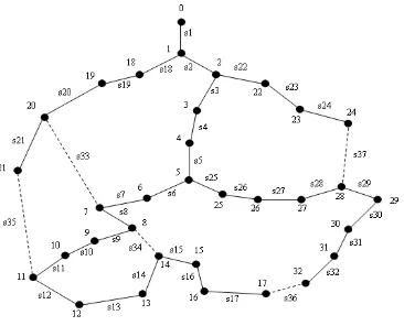
In order to see the satisfactory effectiveness and efficiency of the proposed method, IEEE 32-bus radial distribution system was used for the case study. Simulation has been conducted for both single and multi-objective modes with stochastic structure. The testing system includes two feeders and five branches. Nominal voltage of the system is 12.66 kV. Single line diagram of the testing system is shown in Figure 1. As will be seen from the Figure, the ties are shown dotted line. About the proposed modified firefly

algorithm, the number of particles iterations is assumed 20 and stopping criterion is considered 100 iterations. This study has been performed to solve DFR problem at the start of optimization by modified single-objective firefly algorithm for each objective function. The following sections discuss the simulation results at 32-bus test system, in single-objective and multi-objective modes and in tables and graphs, the results will be compared. In all cases, success and effectiveness of the proposed approach is evident. Table 1 shows the optimization results of the system active power losses.

Figure 1: A schematic linear view of IEEE 32-bus network

Table 1: optimization of objective function of active power losses by the proposed method on test network in

deterministic structure (without turbine)

Open keys losses

[KW] method

s7,s9,s14,s32,s37 139/53 PSO–ACO [19]

s7,s9,s14,s32,s37 139/53 DPSO–HBMO [20]

s7,s9,s14,s32,s37 139/53 McDermott et al [21]

s7,s9,s14,s32,s37 139/53 Vanderson Gomes[22] s7,s9,s14,s32,s37 139/53 PSO-SFLA [23]

s7,s10,s14,s32,s37 140/26 Shirmohammadi [5]

s7,s9,s14,s32,s37 139/53 MFA

286 Table2: emission objective function factors for different

distributed generation sources

Emission factor in (kg/MWh) Wind

turbin e

Micro-turbine

Gas

turbine Network

Polluta nt

0 0/1995 0/013

6 2/2952 NOx

0 723/93 488/9

7 921/25 CO2

0 0/0036 0/002

7 3/5834 SO2

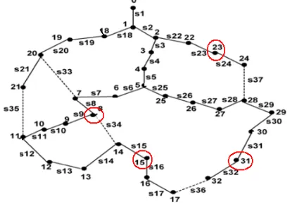
So far the calculations have been carried out to demonstrate the appropriate response of the proposed evolutionary algorithm. Also in Table 1, the presence of wind turbines on the network is neglected. Then we study and apply the proposed stochastic structure based on load flow. Location of wind turbines in the network is shown in Figure 2.

Figure 2: linear schematic view of IEEE 32 -bus network with wind turbines (the red dots)

Table 3 will show results of the multi-objective optimization of objective functions separately with wind turbines in the network. Here the possible proposed framework based on probabilistic load flow has been used.

Table 3: results of the multi-objective optimization with wind turbines in the proposed stochastic structure

Keys position optimal

solution method

Objective function

s6,s14,s35,s17,s37 101/12192

GA Power

losses [kW]

s7,s14,s35,s32,s37 101/39677

PSO

s7,s14,s10,s30,s37 550231

/ 94 MFA

s6,s11,s35,s36,s37 154/11901

GA Cost

[$] PSO 154/09343 s7,s14,s10,s32,s37 s7,s14,s10,s30,s37 153/86291

MFA

s6,s14,s21,s26,s37 37168/231

GA

Pollution [kg]

s4,s14,s21,s26,s37 37167/985

PSO

s33,s14,s35,s36,s22 36802/517

MFA

As can be seen in table (3), the presence of wind power sources in the network has been able to significantly reduce the objective functions. In terms of optimization, superior performance of the proposed algorithm over PSO and GA is well observed. To see the effect of taking the wind fluctuations in equations, table (4) shows the standard deviation values of each function before and after reconfiguration.

Table4: standard deviation values of the objective functions in the presence of wind turbines in the proposed stochastic

structure

Pollution [kg] Cost [$] Power losses [kW] Standard deviation

468/4523 6/7431

4/2732 Initial σ

462/285 5/3021

3/1234 final σ

It is observed that the standard deviation value of each objective function has been reduced after optimization and, in fact, the reliability of the results has been increased.

7. Conclusions

In this paper, the idea of possible load flow has been used for modeling the uncertainty caused by fluctuations in wind speed and prediction error of active and reactive loads. Also for simultaneous optimal management of 3 objective functions, the idea of Pareto optimal points was used. For space exploration of the problem, a powerful optimization algorithm based on modified firefly algorithm was presented. The simulation results show the superiority of the proposed algorithm over other well-known algorithms in the field of reconfiguration. Also, the proposed stochastic structure has the proper power to consider the uncertainty of random variables of the problem so that by reducing the standard deviation of the objective functions, it has led to increase the reliability of the results. The simulation results showed that the presence of wind turbines as a source of new energy in the network could lead to: 1) reduce active power loss, 2) reduce overall costs and 3) reduce total emissions produced by the network.

References

[1] Shin-An Y., Chan-Nan L. (2009), ―Distribution Feeder Scheduling Considering Variable Load Profile and Outage Costs‖, IEEE Transactions on Power Systems, Vol. 24, No. 2.

[2] Vanderson Gomes. F., Carneiro.S., Pereira. J. L. R., Garcia Mpvpan, and RamosAraujo, L. (2005), ―A new heuristic reconfiguration algorithm for large distribution systems‖, IEEE Transactions on Power Systems, vol. 20 no.3, pp.1373–1378.

[3] Zheu Q., Shirmohammadi D., and Liu W.H., ―Distribution Feeder Reconfiguration for Service Restoration and Load Balancing‖, IEEE Trans. On Power System, vol. 12, no.2, pp. 724-729.

287 urban power distribution system‖ Proceedings of

5th Power System Computation Conference (PSCC), Cambridge, UK, pp. 1-18.

[5] Shirmohammadi D., Wayne Hong H. (1989), ―Reconfiguration of Electric Distribution Network for Resistive Losses Reduction‖, IEEE Trans. on PWRD, pp. 1402-1408.

[6] Baran M.E., Wu F.F. (1989), ― Network reconfiguration in distribution systems for loss reduction and load balancing‖, IEEE Trans. Power Delivery 4 (2) 1401–1407.

[7] Schmidt H.P. and Kagan N. (2005), ― Fast reconfiguration of distribution systems considering loss minimization‖, IEEE Trans. Power Syst. vol. 20 no.3, pp.1311–1319.

[8] Jeon Y.J. , Kim J.C. , Kim J.O. , Shin J.R., and Lee K.Y. (2002), ― An Efficient Simulated Annealing Algorithm for Network Reconfiguration in Large-Scale Distribution Systems‖, IEEE Transaction on Power Delivery. vol.17 no.4, pp.1070–1078.

[9] Augugliaro A., Dusonchet L., Ippolito M., and Sanseverino E.R. (2003), ―Minimum Losses Reconfiguration of MV Distribution Networks Through Local Control of Tie-Switches‖, IEEE Transaction on Power Delivery, vol.18, no.3, pp. 762–771.

[10]Das D. (2006), ―A Fuzzy Multi-Objective Approach for Network Reconfiguration of Distribution Systems‖, IEEE Transaction on Power Delivery. vol. 21, no.1, pp.202–209.

[11]Rao R.S., Narasimham S.V.L., Raju M.R., and Rao A.S. (2011), ―Optimal Network Reconfiguration of Large-Scale Distribution System Using Harmony Search Algorithm‖, IEEE Transactions on Power Systems. vol. 26 no.3, pp.1080-1088.

[12]Olamaie J., Niknam T., Gharehpetion G. (2012), ―Application of particle swarm optimization for distribution feeder reconfiguration considering distributed generators,‖ Appl Math Comput; 20(1):575–86.

[13]Niknam T. (2011), ―Application of honey-bee mating optimization on state estimation of a power distribution system including distributed generators,‖ J Zhejiang Univ Sci;9(12):1753–64.

[14]Malekpour A.R. , Niknam T. , Pahwa A. , and Kavousi Fard A. (2012), ― Multi-objective Stochastic Distribution Feeder Reconfiguration in Systems with Wind Power Generators and Fuel Cells Using Point Estimate Method,‖ IEEE Trans. Power Systems, 1483 – 1492.

[15]Rosenblueth E. (2003), ―Point estimation for probability moments,‖ Proc. Nat. Acad. Sci., vol. 72, no. 10, pp. 3812–3814.

[16]T. Apostolopoulos, A. Vlachos, ―Application of the Firefly Algorithm for Solving the Economic Emissions Load Dispatch Problem,‖International Journal of Combinatorics, ID: 523806 (2011) 1-23

[17]X. S. Yang, ― Nature-Inspired Metaheuristic Algorithms,‖ Frome: Luniver Press. (2009), ISBN 1905986106.

[18]Horn J., Nafpliotis N., and Goldberg D.E. (2007), ―A Niched Pareto Genetic Algorithm for Multiobjective Optimization,‖ IEEE World Congress on Computational Intelligence, Piscataway, NJ. Vol. 1, pp. 82-87.

[19]Niknam T. (2010), ―An efficient hybrid evolutionary based on PSO and ACO algorithms for distribution feeder reconfiguration,‖ European Trans on Elect Power, vol. 20, pp. 575 – 590.

[20]Niknam T., Taheri S.I. , Aghaei J., Tabatabaei S., Nayeripour M. (2011), ― A modified honey bee mating optimization algorithm for multiobjective placement of renewable energy resources,‖ Applied Energy , vol. 88 , pp. 4817-4830.

[21]McDermott T.E., Drezga I., Broadwater R.P. (1999), ―A heuristic nonlinear constructive method for distribution system reconfiguration,‖ IEEE Trans on Power Sys, vol. 14, pp. 478 – 483, 1999.

[22]Carneiro S.J, Pereira J.L., Vinagre M.P., Garcia P.A., Araujo L.R. (2005), ―A New Heuristic Reconfiguration Algorithm for Large Distribution Systems,‖ IEEE Tran on Power sys, vol. 20 , pp. 1373 – 1378.