Abstract: We present ÉIRE Mod, a quarterly DSGE model developed for macroeconomic policy analysis in Ireland. We simulate productivity and wage and price mark-up shocks to mimic the impact of various structural reforms aimed at improving the efficiency and competitiveness of the Irish economy. We find that all the structural reforms lead to an increase in aggregate output. However, depending on the source of the shocks, there are important differences in the transmission channels and the effect on employment and external competitiveness. This work is the first step towards the development of a suite of DSGE models for Ireland. Extensions of the core ÉIRE Mod detailed here will further enhance its analytic capabilities.
I INTRODUCTION
D
ynamic Stochastic General Equilibrium (DSGE) models have become increasingly popular tools for policy analysis in Central Banks and other policymaking institutions. These models formalise the behaviour of economic1
ÉIRE Mod: A DSGE Model for Ireland
DARAGH CLANCY*
European Stability Mechanism, Luxembourg
ROSSANA MEROLA†
International Labour Organisation, Geneva
Acknowledgements:This work was conducted while the authors were members of the Macro Modelling Project. However, the views contained here are those of the authors and not necessarily those of their past or present institutions. The authors thank two anonymous referees, the associate editor John McHale, Jaromir Beneš, Dawn Holland, Luca Onorante, Gerard O’Reilly, all past and present members of the Macro Modelling Project team and seminar participants at the Central Bank of Ireland and The Economic and Social Research Institute. However, all remaining errors are our own.
agents based on explicit microfoundations and rational forward-looking expectations. As a result, DSGE models are less prone to the Lucas critique (Lucas, 1976) than traditional macroeconometric models, and therefore provide a powerful framework for conducting policy scenario analysis.1We develop a quarterly DSGE model for Ireland, ÉIRE Mod (Elementary Irish Real Economy Model). We design the model’s underlying structure to replicate the highly open nature of the Irish economy. Moreover, we calibrate the model to match the steady-state ratios of key macroeconomic variables, using long-run averages (1960-2010) from National Account data. To highlight the usefulness of the model for policy analysis, we examine the impact of various structural reforms on the Irish economy. This is in the spirit of existing work that examines the short- and long-run macroeconomic effects of structural reforms using DSGE models.2
The simulation of these shocks highlights the transmission channels through which such reforms would affect the Irish economy. Structural reforms have been on the Irish policy agenda since the beginning of the decade, as the financial crisis exposed the loss of competitiveness suffered during the excesses of the housing boom. Successive policy documents, from Europe 2020 to the Financial Assistance Programme, the Programme for Government and the Medium-Term Economic Strategy (MTES), all call for the introduction of structural reforms to boost the sustainable growth potential of the Irish economy. These documents emphasise that a series of measures designed to reform the Irish labour and product markets could deliver medium-term growth through productivity gains. Specifically, we analyse the effect of increases in productivity (i.e., R&D investment) and competitiveness (i.e., limiting wage bargaining and reducing barriers to entry for new firms). Our results show that, although all the reforms boost aggregate output, differing transmission channels for the shocks have contrasting implications for Ireland’s external competitiveness and employment. Given the MTES commits to a strategy of export-led growth and full employment, a careful assessment of the reforms implemented under this programme is necessary to ensure that they do not lead to counter-productive effects in the export sector and employment.
The following section provides an overview of the model, while Section III describes the calibration process. Section IV details the simulations of various structural reforms aimed at improving the efficiency and competitiveness of the Irish economy. These illustrate the transmission channels through which
1 For a more exhaustive discussion, see Tovar (2008) and Vetlovet al.(2010).
structural reforms affect the Irish economy. The final section summarises the main results and briefly discusses planned extensions to the model framework.
II THE MODEL
We consider a two-sector small open economy within a monetary union.3 Agents in the economy are households, firms producing non-tradable goods and exports, and retailers who import goods from abroad for sale on the domestic market. We include New Keynesian features such as sticky prices and wages, and thus accurately replicate the sluggish reactions of economic variables, such as inflation and output, found in the empirical literature.4Formally, we assume that labour and goods markets are characterised by a monopolistically competitive structure. Households and firms use their bargaining power to set their wages and prices as a mark-up over their respective marginal costs, subject to the (downward sloping) demand curves for their produce. We follow Benešet al.(2014) and assume that the locus of the demand curve, determined by the aggregate price and quantity, is not internalised by the optimising (representative) agent but set equal to its individual counterpart in symmetric equilibrium.5
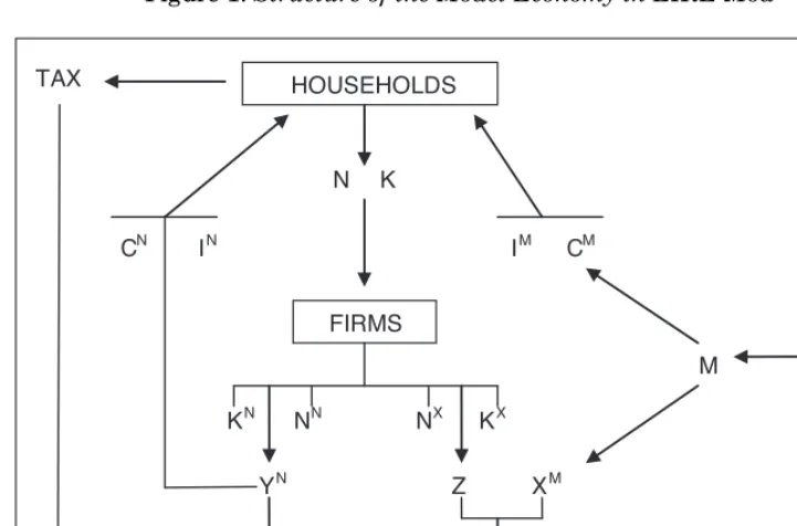
Variables not internalised (i.e., taken as given) by optimising agents, such as external habit formation in consumption, are marked with a bar. Deviations from steady-state wages and prices are subject to quadratic adjustment costs, modelled à la Rotemberg (1982). As a result, wages and prices adjust only gradually in response to a shock to demand or marginal cost. We introduce real rigidities via external habit formation in consumption and investment adjustment costs. We account for Ireland’s membership in the European Monetary Union in a number of ways. We assume the European Central Bank exogenously sets the nominal interest rate, which therefore does not react to domestic economic developments. The government raises revenues via taxes to finance exogenous public spending, and pursues a balanced budget policy. A flow-chart of the model economy is depicted in Figure 1, and we provide a glossary of the model variables and parameters in the Appendix.
3See Devereuxet al.(2006) and Merola (2010) for further analytical details on two-sector small open economy models, and Lane (2001) for a survey of the New Open Economy Macroeconomics Synthesis, which is the theoretical foundation behind this model.
4See Woodford (2003) and Galí (2008) for textbook treatments of New Keynesian theory and its incorporation in modern macroeconomic models.
2.1 Households
Households gain utility from consumptionCtand disutility from labourNt. They maximise their lifetime utility:
` 1
E0
o
bt3
(1 –c) log (C t–cC—
t–1) – –––––Nt1+h
4
(1)t=0 1 + h
where b is the discount factor, c is the degree of habit persistence in consumption, (1- c) is a scale factor which guarantees that the marginal utility of consumption in the steady state is independent from the habit parameter and his the labour supply elasticity. Maximisation of the utility function is subject to a budget constraint:
1 1 1
Bt+PtCt+PtIIt
3
1-–xI(WtI)2
4
+PtNYtN3
–xN(WtN)24
+PtMMt3
–xM(WtM)22 2 2 1 1 +PtXXt
3
–xX(WtX)2
4
=RtBt-1+RtKKt-1+WtNt3
1 – –xW (WtW)24
(2)2 2
+ Pt- Qt,
Figure 1: Structure of the Model Economy in ÉIRE Mod
NX KN
HOUSEHOLDS
M IM
CN
N K
NN KX
A B R O A D
YN Z XM
X FIRMS
IN CM
whereBtare bond holdings,Rtis the nominal (risk-free) interest rate on these assets, Ptare profits from firms (whom the households are assumed to own) and Qtare lump sum taxes paid to the fiscal authority. The budget constraint requires that households’ bond holdings, tax liabilities and purchase of consumption goods (at pricePt) and investment goodsIt(at pricePtI) must be covered by their labour incomeWtNt, capital incomeRtKKtand dividends from firms Pt. Factor inputs are paid at the wage rateWtand the rental rate of capitalRtK. Households’ resources in the budget constraint are net of adjustment costs. Adjustment costs, not internalised by households but instead rebated in lump-sum form, arise from deviations in non-tradable good price inflation
pN p
tP
M
WtN = log ––––, import sector price inflation WtM = log –––– and quantity
pN
t–1 pP
M
t–1 Xt
adjustment in the export sector WtX = log––––.6In addition, households face Xt–1
It pWt
adjustment costs in investment WtI= log–––and in wage inflation WtW= log––––.
It–1 pW
t–1 In all cases, the size of these costs are controlled by adjustment cost parameters
xI, xN,xM,xXand xW. Households also take into account a law of motion for
capital:
Kt= (1- d)Kt-1+It. (3) This equation states that the capital stock available at the beginning of period t,Kt, is equal to the capital stock available at the end of period t–1, net of capital stock depreciationdKt-1, where 0< d<1 is the capital depreciation rate, plus the amount of capital accumulated during period t, which is determined by the investment made during period t, It. The first order conditions forBt,ItandKtrespectively are:
Lt=bEtLt+1Rt, (4)
PtK»PtI+xIP
tI(WtI- bEtWtI+1) (5)
Lt+1
PtK» bEt–––– (RKt+1+ (1- d)PKt+1), (6)
Lt
where Ltis the multiplier associated with the budget constraint and the»sign indicates the omission of second- or higher-order terms from the equation.7In symmetric equilibriumCt=C—t, and so the first order condition with respect to consumption is:
1-c
––––––––– = LtPt. (7)
Ct- cC—t-1
2.1.1 Labour supply and wage determination
Households use their monopoly power to set their wages so as to maximise the intertemporal objective function subject to both the budget constraint and a downward-sloping demand curve for their labour:
Wt
Nt=
1
––2
N—t (8)W—t
qW
whereqWis the elasticity of labour demand andm t
W=–––––is a mark-up over
qW– 1
the marginal cost of labour, which follows an autoregressive process:
mWt = (1- rW) mW+rW mW
t-1+ eWt (9)
where mWis the steady state of the mark-up over the marginal cost of labour,
rWis the persistence of the process ande t
Wis a shock to the wage mark-up.
The first order condition for labour, by which households choose the optimal wage, is:
mW t Nth
–––––»1 + (mW t -1)xWW t W -(m
t
W -1)xNbE
tWWt+1 (10) WtLt
and Wt= W—t, Nt= N—t in symmetric equilibrium. The equilibrium condition, Equation (10), represents the New Keynesian wage Phillips curve.8Under full price flexibility (i.e.,xW= 0), households would always set wages as a mark-up
7 Similar to Beneš et al. (2014), we are only interested in the first-order dynamic effects of adjustment costs. We therefore simplify the notation by dropping higher order terms relating to adjustment costs. Since we linearise our model around a first-order approximation of the non-stochastic steady state, this simplification has no effect on the model solution or simulations. Naturally, a desire to examine higher-order approximations of the model would necessitate the inclusion of these additional terms.
8 We have derived all the New Keynesian Phillips curves in the context of the Rotemberg (1982) model of price stickiness. However, similar dynamics emerge under another commonly used model of nominal rigidity due to Calvo (1983).
mW
– ––––––
over the marginal rate of substitution between consumption and labour. Equation (10) implies that wages are set in a forward-looking manner, and are inversely related to both current employment and its expected future path.
2.2 Firms
There are three types of firms. While one locally produces non-tradable goods, another produces exports goods for sale on the international market. A final type imports foreign goods for sale on the domestic market. Firms producing domestic goods and firms importing foreign goods are assumed to face a small direct cost of adjusting their prices. As a result, these firms will only adjust prices gradually in response to a shock to demand or marginal cost. As exporters are assumed to be price takers on the world market, they face quadratic adjustment costs if they want to change their output levels.
2.2.1 Non-tradable good producers
Local producers combine domestic capital,KNt–1, and labour,NtN, using a Cobb-Douglas production function to assemble a non-tradable good:
YtN=AtN(KNt–1)1–gN(NtN)gN (11) where gN measures labour share in the non-tradable sector and A
t N is an
exogenous technology term which follows an autoregressive process:
logAtN=rAlogAN
t–1+ etA (12)
withrA the persistence of the process ande
tA a shock to non-tradable sector
productivity. This shock is sector specific and is identical across all firms in the sector. The local producer optimises the present value of payoffs:
` 1
E0
o
btLt
3
PtNYtN3
1 –xN(WtN)24
–WtNtN–RtKKNt–14
(13)t=0 2
The optimal choice of labour and capital, respectively, is:
gNMC t NY
tN=WtNtN (14)
(1- gN)MC
PtN –qN
Yt=
1
–––2
Y—t (16)P—tN
whereqNis the elasticity of demand for non-tradable goods. Local firms can use
their degree of monopoly power to charge a mark-up over their marginal cost. Given that PtN=P—tNin symmetric equilibrium, the optimal price is set according to:
mtNMCtN
(mtN-1)xNW
tN»(mtN-1)xNbEtWNt+1+
1
–––––––-12
(17) PtNqN
where mtN= ––––– measures the monopolistic mark-up in this sector, which
qN -1
follows an autoregressive process:
mtN= (1- rN)mN+rNmN
t–1+etN (18)
where mN is the steady state of the mark-up in the non-tradable sector, rN
represents the persistence of the process andetNis a shock to the non-tradable price mark-up. The equilibrium condition, Equation (17), represents the New Keynesian Phillips curve, which describes how prices are set depending on current inflation, expected future inflation and the current deviation of marginal cost from marginal revenue. Under full price flexibility (i.e.,xN= 0),
the firm would always set prices as a mark-up over the marginal cost (which equals the marginal revenue). However, with quadratic costs of changing nominal prices, this practice is costly. Current inflation is increasing in expected future inflation, because in the presence of nominal price adjustment costs, a firm expecting higher inflation in the future may want to smooth the necessary price adjustments over time by beginning to raise prices in the current period.
2.2.2 Importers
The import sector consists of firms that buy a homogeneous good in the world market, and use a branding technology to convert the imported goods into differentiated products, which are then sold to local households. It is assumed a set of monopolistic domestic importers purchase the foreign good at its marginal cost (expressed in domestic currency), MCtM =PtM*St, wherePtM* is
the world import price expressed in foreign currency and Stis the nominal exchange rate. For a small open economy,PtM* is taken as given. Import firms
PtM –qM
Mt=
1
–––2
M—t (19)P—tM
qM
to charge a mark-upmM = –––––– over this price, with qM representing the
qM– 1
elasticity of demand for imported goods. The monopolistic mark-up in this sector follows an autoregressive process:
mtM= (1- rM)mM+rMmM
t–1+ etM (20)
wheremMis the steady state of the mark-up in the import sector, rMis the
persistence of the process and etM is a shock to the import price mark-up. AssumingPtM= P—tMin symmetric equilibrium, these goods are then sold on the domestic market at pricePtM:
mtM MCtM
1
–––––––2
»1 + (mtM– 1) xMWtM-(mtM -1)xMbEtWMt–1 (21) PtM
with this price setting mechanism following the same rationale to that described previously for the non-tradable good sector. Local currency price stickiness allows for an incomplete exchange rate pass-through, and thus there is some delay between movements in the terms of trade and the adjustment of imported goods prices.
2.2.3 Export good producers
Competitive local exporters combine domestic labour and fixed capital
K—tX-1to create a tradable good using a Cobb-Douglas technology:9
Zt=AtX(K—tX-1)1–gX(NtX)gX (22) wheregX measures labour intensity in the export sector and A
t
X is a sector
specific exogenous technology term which follows an autoregressive process:
logAtX=rXlogAX
t-1+ etX (23)
9 The capital input decisions of export sector firms are not necessarily made domestically in small open economies with a large amount of Foreign Direct Investment (FDI) (for a detailed discussion, see Bradley and Fitzgerald, 1988 and 1990). Consistent with this, export firms concentrate solely on the minimisation of labour costs and capital follows an autoregressive process logK–tX=rKlog
K–t–X1+eKt, whererKis the persistence of the process andetKis a shock to the export sector’s capital
with rX the persistence of the process and e t
X a shock to export sector
productivity. Re-exportsXtM, which are goods purchased from abroad but not intended for sale in the domestic market, are combined with the locally produced tradable goods Zt to produce final export goods using a Leontief production function:
Zt XtM
Xt= min
5
––––––, –––6
. (24)(1- a) a
The large size of the multinational sector in Ireland makes this import content of exports channel very relevant for policy analysis.10By considering the international fragmentation of the export goods production process, this feature can account for the reliance of exports in Ireland on imported components. For any given level of output, the inputs in the final export good
Xtare combined in proportions fixed by a parameter a:
Zt= (1- a)Xt (25)
XtM=aXt. (26)
This assumption of fixed proportions in the export bundle means that changes in relative prices should not overly influence the use of imported intermediate goods in the production of the final export good. In a small open economy such as Ireland, the imported component is often not produced within the country, and so is irreplaceable from domestic sources. With capital fixed, domestic firms producing the tradable good Ztminimise their costs:
`
E0
o
bt Lt
3
PtXXt-WtNtX-RtKK —Xt-1
4
. (27)t=0
This optimisation choice only considers the domestic component, as the imported component is set to a fixed proportion of the final export good. The optimal choice of labour in this sector is derived from:
gX MC t Z Z
t=WtNtX. (28)
The exporters marginal cost of production is:
MCtX= (1- a)MCtZ+aPtM*St (29) whereMCtZis the marginal cost of locally-produced tradable goods used in the final export good production process, whilePtM*Stis the world import price defined previously. In line with our small open economy assumption, Irish exporters are assumed to be price takers on the world market (i.e.,PtXis taken as given). Export firms, therefore, only decide on the quantity to produce at a given price. After substituting the total production cost into the exporters’ pay-offs, we can derive the following first-order condition for the optimal level of exports:
PtX
––––»1 +xXW
tX- bEtWXt–1 (30) MCtX
which again contains a forward-looking component relating current output changes to underlying marginal costs and expected future adjustment costs. Consistent with the small open economy assumption, foreign inflation is exogenously given and an increase in Irish exports does not influence world prices. Therefore, endogenous changes in Ireland’s external competitiveness are driven by domestic factors.
2.3 Net Foreign Asset Position
Given the small weight of Ireland in the euro area (approximately 1 per cent), domestic developments are too small to affect area-wide macroeconomic aggregates. Therefore, the domestic interest rate,Rt, is assumed to be tied to the exogenously set euro area interest rateRt*:11
EtSt+1
Rt=Rt* –––––eF (31)
St
whereeFis a debt elastic risk premium used to close the model, as in
Schmitt-Grohe and Uribe (2003). This premium is defined as:
Bt
eF=p
1
––– – log z2
(32)Yt
steady-state level. The implication of this model feature is that households have as much access to (foreign) funds as they desire, but the more they borrow the greater the premium they will be charged. This ensures that debt will not explode, as households will eventually try to reduce their debt back to the steady-state level to ensure they will not be charged this additional premium. This feature ensures the model is stationary (i.e., the model returns to the steady state following a temporary shock), a notoriously difficult task in small open economy models.
Consistent with the small open economy assumption that the rest of the world is taken as given and not modelled explicitly, the country’s net foreign assets (NFA) evolve according to:
Bt=Bt-1Rt-1-(PtXXt-PtMMt) (33) with the interest households earn from bond holdings defined by Rt-1since savings accrue a nominal amount with certainty (i.e. a zero coupon bond).12 The evolution of NFA of the home country is determined by the aggregate stock of last period’s NFA times the interest rate, plus (minus) the trade surplus (deficit). Since both importers and exporters are assumed to be price takers on the world market, and the the nominal exchange rate is fixed in line with Ireland’s small weight in euro area aggregates, we abstract from valuation effects and implicitly assume that the trade balance is equal to the current account balance.
2.4 Policy Authorities
With monetary policy exogenous, instead of a Taylor rule we assume that a fixed exchange rate is maintained (i.e., the nominal exchange rate equals one). The fiscal authority is stylised, and is primarily included in order to obtain a more accurate calibration of key steady-state ratios. Government spending is specified as a fraction,g, of steady-state nominal outputY—:
Gt=gY— (34)
and is assumed to consist entirely of domestically produced non-tradable goods. A balanced budget is ensured in every period by a lump-sum tax (transfer) Qt
that offsets any fiscal deficit (surplus):
PtNGt= Qt. (35)
2.5 Market Clearing Conditions
The final consumption goodCtand investment goodItare an aggregate of locally produced non-tradables and imports, bundled in fixed proportions:13
Ct=wCC t
M+ (1- wC)C t
N (36)
It=wI I t
M+ (1- wI) I t
N (37)
wherewCandwIare the share of imports in final consumption and investment
goods respectively. The real prices of the consumption and investment goods are derived by imposing the following conditions:
PtCt=PtNCtN+PtMCtM (38)
PtIIt=PtNItN+PtMItM. (39) In equilibrium, the final goods markets clear when the demand from households and the rest of the world is matched by the production of final goods firms. The bond market is in equilibrium when the positions of the export and importing firms equals the households’ choice of bond holdings (i.e., a trade surplus is necessary to pay down borrowings from abroad). The clearing conditions for the non-tradable goods, import, labour and capital markets are, respectively:
YtN=CtN+ItN+Gt (40)
Mt=CtM+ItM+XtM (41)
Nt=NtN+NtX (42)
Kt=KtN+K—tX (43) where capital in the export sector is fixed. Given that all households choose identical allocations in equilibrium, the aggregate quantities are expressed in domestic per capita terms. Adding the budget constraint of households and the entrepreneurs in each sector would allow us to derive the aggregate consolidated balance of payments condition for the economy. The economy’s aggregate resource constraint is therefore:
III CALIBRATION
We model the specific nature of the Irish economy within the context of the EMU. The calibration process involves the specification of values for steady-state (long-run) ratios, and model parameters that govern the model’s dynamic adjustment to shocks. These values are provided in Tables 1 and 2. We target key steady-state ratios in order to resemble the underlying structure of the Irish economy. However, given the large fluctuations in the Irish economy since the foundation of the state, the elicitation of appropriate steady-state values is difficult. We choose a calibration based on the long-run averages (1960-2010) from the national accounts statistics, as gathered from the Economic and Social Research Institute (ESRI) model database. This data allows for the longest possible time horizon to be used.14
Table 1: Calibrated Model Steady-States (as Percentage of GDP)
Per Cent
Private Consumption 64.0
Private Investment 17.4
Public Expenditure 16.8
Exports 69.7
Imports Total 67.9
Imports for Consumption 23.2
Imports for Investment 9.8
Imports for Re-export 34.9
Net exports 1.8
Table 2: Calibrated Model Parameters
Households
Discount Factor 0.9926
Frisch Elasticity 1
Consumption Habit Persistence 0.80
Consumption Import Share 0.29
Investment Import Share 0.48
Capital Depreciation Rate 0.04
Wage Rigidity 25
Investment Rigidity 3
Debt Convergence 0.02
Table 2: Calibrated Model Parameters (Contd.)
Export Sector Firms
Labour Share 0.40
Capital Share 0.60
Output Rigidity 5
Non-tradable Sector Firms
Labour Share 0.70
Capital Share 0.30
Price Mark-up 0.10
Price Rigidity 25
Import Sector Firms
Price Mark-up 0.10
Price Rigidity 15
We assume the economy starts out in a steady state with zero consumption growth. Thus, the interest rate must equal the rate of time preference. We set the household’s subjective discount factor consistent with an (annualised) interest rate of 3 per cent. The nominal output shares of government expendi -tures (16.8 per cent) and investment (17.4 per cent) are set to the respective domestic demand shares of public consumption and gross capital formation.15 In the steady state, the trade balance simply covers net foreign interest payments. We therefore calibrate external debt to replicate steady state net exports to GDP of 1.8 per cent. We then set the share of consumption (64.0 per cent) equal to the residual of the sum of the remaining output shares.
However, data averaged over the very long run may not be as useful in capturing Ireland’s international trade relations. Therefore, the imported intermediate inputs in exports is set at 50 per cent, in line with OECD estimates using input-output (I/O) tables for the period 1995-2010. The share of imports in the aggregate consumption (29 per cent) and investment (48 per cent) baskets are based on the latest available (2008) final use breakdown of imports from the Central Statistics Office I/O tables. These latter features ensure that the model captures the highly open nature of the Irish economy. The factor-intensity parameters are important in determining the dynamics of the model. As only labour is mobile between the non-tradable and export
sectors, the impact of productivity and terms of trade shocks will depend on the differing labour intensity of these sectors. Several Irish studies (e.g., Bermingham, 2006) have found that the non-traded sector is more labour intensive than the export sector. Following these studies, as well as examining sectoral data from the ESRI macro economic database, the labour share of export and non-tradable goods is set to 40 per cent and 70 per cent respectively. Accordingly, the total share of labour in output is 55.4 per cent.
Following the New Keynesian tradition, the model uses real and nominal rigidities in order to match the sluggish reaction of prices, wages and other economic variables found in macroeconomic data. However, data on such features is limited or non-existent in the case of Ireland. Therefore, the calibration process involved identifying common values in the literature and recursively updating them when the impulse response functions (IRFs) did not correspond to well-known macroeconomic theory regarding the business cycle (see, for example, King and Rebelo, 1999).
Druantet al.(2009) identified a relatively high degree of friction in the Irish goods and labour markets, implying a lower level of competition. However, Keeneyet al.(2010) and Keeney and Lawless (2010) note that this may be due to the boom in Ireland during the period in which the survey used by Druantet al.(2009) took place. Keeney and Lawless (2010) find that, despite the lack of wage decreases during the period, Irish firms had the least issue with regulations of all euro area countries surveyed. This finding, coupled with evidence of wage decreases since the onset of the financial crisis, suggests greater flexibility in the labour market. In light of such offsetting evidence for goods and labour market flexibility, we decided to keep price and wage mark-ups at standard values found in the literature (e.g., Ireland, 2001; Devereuxet al., 2006; Keen and Wang, 2007).
IV SIMULATION EXERCISES
low firm birth and death rates indicating the Irish enterprise sector is not as dynamic as other OECD countries. Cumbersome licence and permit regulations, the use of market power by large firms to dictate long credit periods to SME suppliers and a high-cost legal system are cited as factors reducing enterpeneurship. Product market reforms reducing barriers to entry for new non-tradable firms could increase competitiveness in this sector. With a focus on export-led growth, the MTES re-confirms the commitment made under the EU/IMF Programme to remove restrictions to trade and competition in sheltered sectors, such as the legal, medical and pharmaceutical professions. These should notionally increase price and wage competitiveness in these sectors. Increased innovation is encouraged through tax credits for R&D spending. This research should manifest itself in the improved productivity of Irish-based firms, thereby boosting their external competitiveness.
To highlight the usefulness of the ÉIRE Mod for policy analysis, we examine the impact that such structural reforms could have on the Irish economy. However, DSGE models are too stylised to explicitly feature some of the nuanced measures proposed in these policy documents. Instead, these simula -tion exercises are an illustrative example of the use of ÉIRE Mod for policy analysis. In order to proxy the beneficial effect of an increase in innovation, we implement an exogenous productivity improvement shock through an increase in the production function efficiency term. To replicate the macroeconomic impact of pro-competition policies, we simulate shocks that reduce the mark-up of wages and non-tradable prices over their marginal costs. These last two simulations mimic an increase in wage competitiveness, and a reduction in the barriers to entry for new firms respectively. We then compare the dynamic reaction of our model to these structural reforms to those found in the Irish theoretical and empirical literature. This benchmarking of the model results against the empirical evidence is a particularly important component in assessing a model’s suitability for policy analysis.
We simulate the model using Dynare (Adjemian et al., 2011). The (stochastic) shocks are temporary and hit the economy at the initial timet= 1, with the persistence of the shock equal to 0.90 in all cases. As the model is quarterly, the impulse response functions represent the dynamic reaction of the model over 40 periods (i.e., 10 years).
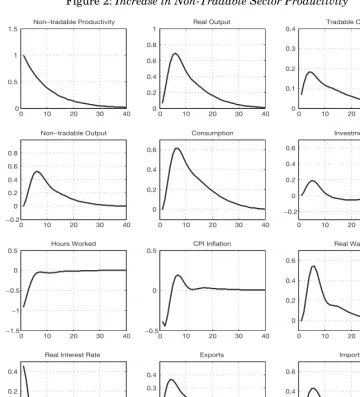
4.1 Effects of Increased Innovation
positive impact on output in both the non-tradable and export sectors. Higher productivity implies lower marginal costs, which feed into lower prices. The lower inflation rate pushes up real wages. As the monetary union nominal interest rate has a minimal reaction to Irish inflation, the real interest rate increases. However, consumption increases as a result of higher labour income and the lower price of domestic goods. Higher efficiency reduces labour demand, with firms replacing labour with capital in the production process. As a result, employment (i.e., hours worked) shifts downwards. This matches empirical evidence on the labour response to technology shocks first provided by Galí (1999) and later replicated by Francis and Ramey (2005) amongst others. Investment, which is more attractive following the shock due to the increased marginal product of capital, initially increases to facilitate the expansion in output. However, over the medium term, the income effect from a steady upturn in employment and the higher real wage rate means that consumption is brought forward at the expense of reduced investment.
The productivity shock, by decreasing marginal costs in the non-tradable sector, makes domestically produced goods relatively less expensive and induces households to substitute imported goods with domestic goods. The change in relative prices discourages imports and improves the trade balance on impact. However, imports rebound relatively quickly, as they represent a large component of final export goods. There is increased production in the export sector as lower domestic costs (from reduced competition for factor inputs by non-tradable sector firms) increases the competitiveness of exporters.
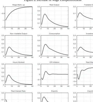
4.2 Effects of Labour Market Reforms: Increased Wage Competitiveness
Figure 3 shows the dynamic impact of increasing wage competitiveness due to the reduction in the degree of monopoly power of workers or trade unions. This scenario is modelled as a transitory negative 1 per cent shock to the wage mark-upmtW. A decrease in the wage mark-up results in lower production costs in both the non-tradable and export sectors through lower wages.16 Non-tradable sector firms pass on these gains to consumers through lower prices. However, export firms are price takers and therefore cannot pass on these cost decreases. The higher demand for non-tradable goods means that firms increase their labour demand and employment increases to produce this extra output. Lower costs also enable export firms to produce more output. However, the effect is muted relative to the non-tradable sector who have now reduced their prices.
Figure 2: Increase in Non-Tradable Sector Productivity
0 10 20 30 40
0 0.5 1 1.5
Non−tradable Productivity
0 10 20 30 40
0 0.2 0.4 0.6 0.8 1 Real Output
0 10 20 30 40
0 0.1 0.2 0.3 0.4 Tradable Output
0 10 20 30 40
−0.2 0 0.2 0.4 0.6 0.8 Non−tradable Output
0 10 20 30 40
0 0.2 0.4 0.6
Consumption
0 10 20 30 40
−0.2 0 0.2 0.4 0.6 Investment
0 10 20 30 40
−1.5 −1 −0.5 0 0.5 Hours Worked
0 10 20 30 40
−0.5 0 0.5
CPI Inflation
0 10 20 30 40
0 0.2 0.4 0.6
Real Wage
0 10 20 30 40
−0.2 0 0.2 0.4
Real Interest Rate
0 10 20 30 40
−0.1 0 0.1 0.2 0.3 0.4 Exports
0 10 20 30 40
0 0.2 0.4 0.6
Imports
costs, but then eventually overshoots in the medium run due to the higher import prices. This increase in imports is necessary in order to satisfy the boost in the export sector output, which employs intermediate imported goods as inputs.
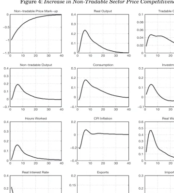
4.3 Effects of Product Market Reforms: Reducing Barriers to Entry
The effects of product market reforms in the non-tradable sector are detailed in Figure 4. The shock is modelled as a temporary negative 1 per cent
Figure 3: Increase in Wage Competitiveness
0 10 20 30 40
−1.5 −1 −0.5 0
Wage Mark−up
0 10 20 30 40
0 0.1 0.2 0.3 0.4 0.5 Real Output
0 10 20 30 40
−0.1 0 0.1 0.2
Tradable Output
0 10 20 30 40
0 0.1 0.2 0.3 0.4 0.5 Non−tradable Output
0 10 20 30 40
0 0.1 0.2 0.3 0.4 Consumption
0 10 20 30 40
−0.1 0 0.1 0.2 0.3 0.4 Investment
0 10 20 30 40
0 0.1 0.2 0.3 0.4 0.5 Hours Worked
0 10 20 30 40
−0.2 −0.1 0 0.1 0.2 CPI Inflation
0 10 20 30 40
−0.5 −0.4 −0.3 −0.2 −0.1 0 0.1 Real Wage
0 10 20 30 40
−0.1 0 0.1 0.2
Real Interest Rate
0 10 20 30 40
−0.1 0 0.1 0.2 0.3 Exports
0 10 20 30 40
Figure 4: Increase in Non-Tradable Sector Price Competitiveness
0 10 20 30 40
−1.5 −1 −0.5 0
Non−tradable Price Mark−up
0 10 20 30 40
0 0.1 0.2 0.3 0.4 Real Output
0 10 20 30 40
0 0.02 0.04 0.06 0.08 0.1 Tradable Output
0 10 20 30 40
−0.1 0 0.1 0.2 0.3 0.4 Non−tradable Output
0 10 20 30 40
−0.1 0 0.1 0.2 0.3 Consumption
0 10 20 30 40
−0.1 0 0.1 0.2 0.3 Investment
0 10 20 30 40
0 0.1 0.2 0.3 0.4 Hours Worked
0 10 20 30 40
−0.4 −0.2 0 0.2
CPI Inflation
0 10 20 30 40
0 0.1 0.2 0.3 0.4 0.5 0.6 Real Wage
0 10 20 30 40
−0.2 0 0.2 0.4
Real Interest Rate
0 10 20 30 40
0 0.05 0.1 0.15 0.2 Exports
0 10 20 30 40
0 0.1 0.2 0.3
Imports
leads to higher demand for factor inputs and hence mitigates the negative effect of higher real wages on employment. Overall, product market reforms support higher employment.
The real interest rate increases, as the monetary union nominal interest rate has a minimal reaction to the drop in Irish inflation. Despite this real interest rate increase, consumption increases as result of the lower relative prices of non-tradable goods and the higher labour income from higher wages and hours worked. These two effects dominate the negative effect that higher real interest rates have on consumption.17As resources are partially reallocated to meet the higher demand for non-tradable goods, output in the export sector increases, but to a lesser extent compared to the case of a decrease in the wage mark-up. This is unsurprising given that this price mark-up shock is specific to the non-traded sector, whereas the wage mark-up shock affected the entire economy. The increased demand for factor inputs leads to an increase in the cost of producing export goods, given that export firms are price-takers and hence are unable to adjust their prices to reflect the increase in input costs. This loss of competitiveness dampens the increase in exports. Imports decrease, as foreign goods are now relatively more expensive than domestic non-tradable goods.
4.4 Comparison with the Literature
In order to assess the usefulness of ÉIRE Mod for the analysis of structural reforms in Ireland, we benchmark the model results against similar studies from the Irish theoretical and empirical literature. Our results on the effects of an increase in wage competitiveness are consistent with those obtained by Callaghanet al.(2014) using the ESRI’s HERMESmodel (Berginet al., 2013). The authors find that a decrease in wage competitiveness adversely affects exporters, who as price-takers are unable to pass the increase in costs on to international customers. The loss of competitiveness reduces output and labour demand. Given that the HERMESmodel is symmetric, the opposite should hold for the reverse case where wage competitiveness improves, as is the basis for our simulation. While our results are qualitatively similar, a quantitative comparison is not possible given the differing approaches to modelling the shocks. While we introduce higher competition through a drop in the wage mark-up, Callaghanet al.(2014) model a change in wage competitiveness as a
change in wages not accompanied by a change in productivity. Barry and Devereux (2006) develop a neo-classical growth model to analyse the effects of a beneficial labour market shock that shifts the economy from an initial system of strong unions with monopoly power to a more centralised wage bargaining system. The authors find that this shock reduces wages and raises employment. Consistent with Barry and Devereux (2006), we also find that the productivity shock leads to a higher effect on GDP than the wage competitiveness shock.
Our results on price competitiveness are also consistent with those of Callaghanet al.(2014), who examine a 1 per cent increase in the price level to proxy for a decrease in competition in product markets. This shock is designed to proxy the impacts of policy choices or other adverse market developments such as the creation or facilitation of barriers to entry (regulatory and otherwise), or regulatory actions that act to limit retail price competition. The increase in prices raises firm’s margins, and has a negative impact on consumption despite a rise in nominal wages. On the external side, price-taking manufacturing sector exporters are unable to pass on the increase in wage costs to international customers, and thus reduce their output and demand for labour in Ireland. As a result, GDP falls in real terms and unemployment rises. As with the wage competitiveness shock, the HERMESmodel’s symmetry allows us to compare these results with ours. From a qualitative point of view, these results are consistent with ours. From a quantitative perspective, the Callaghan
et al.(2014) analysis shows that the overall effect of this policy choice would be to reduce GDP in the long run by 0.3 per cent. Total employment falls by onethird of a percentage point in the long run, along with an increase in unemploy -ment. Again, a comparison of the magnitude of our results is not possible, given the alternative approaches to modelling these shocks. While in Callaghanet al.
(2014) reforms affecting competition are modelled through their “second-round effects” on the consumption price, we model a change in competition more directly though a change in firm’s mark-up.
As Ireland is a small open economy, it is essential that the dynamic reaction of the trade balance is consistent with the empirical literature. The negative association between higher economic activity and external competitiveness is a common feature of empirical studies of the Irish economy (see, for example, Berginet al., 2013; Bermingham, 2006; Bermingham and Conefrey, 2014). In fact, Podstawski (2014) provides empirical evidence that this price competitiveness channel has been the most important driver of Irish current account deficits.18Overall, our model dynamics are in accordance with the Irish
theoretical and empirical literature, both in terms of direction and magnitude. We therefore consider our model well-tailored for the Irish economy and useful for counterfactual policy experiments.
V CONCLUSIONS AND FURTHER EXTENSIONS
We develop ÉIRE Mod, a quarterly DSGE model suitable for policy analysis in Ireland. We simulate productivity and wage and price mark-up shocks to mimic the impact of various structural reforms aimed at improving the efficiency and competitiveness of the Irish economy. We find that all the structural reforms lead to an increase in aggregate output. However, depending on the source of the shocks, there are important differences in the transmission channels and the effect on employment and external competitiveness. An increase in non-tradable sector productivity also benefits the tradable sector and supports export-led growth. Real wage income increases due to the large decline in inflation. Facing a relaxed budget constraint, households increase their consumption spending. The higher efficiency in factor input usage, however, reduces labour demand and employment.
This is not the case for the mark-up shocks, where employment expands following the reforms. A reduction in the monopoly power of non-tradable firms makes export-good firms relatively less competitive. This is unsurprising given that this price mark-up shock is specific to the non-traded sector. A reduction in the bargaining power of households in wage negotiations benefits both the tradable and non-tradable sectors, boosts exports and supports opportunities for export-led growth. Given the MTES commits to a strategy of export-led growth and full employment, a careful assessment of the reforms implemented under this programme is necessary to ensure that they do not lead to counter-productive effects in employment and external competitiveness.
barriers to entry in parallel with labour market reforms reverses the wages losses that would result from the latter alone.
This work is a first step toward a suite of DSGE models for Ireland, and illustrates the transmission channels and policy analysis capabilities of ÉIRE Mod. However, there will be a number of extensions to the ÉIRE Mod. Already on the agenda are a financial sector (for greater details, see Clancy and Merola, 2014), a labour market with involuntary unemployment and labour market frictions, a housing supply sector and a detailed fiscal sector. The development of these extensions on a relatively simplistic and consistent core will help with the tractability of the models. Additionally, key aspects from the various extensions could be combined (e.g., the housing and financial sectors) to analyse important transmission mechanisms between these sectors. A further step will be the estimation of ÉIRE Mod. This will permit a historical decomposition of the shocks driving the Irish business cycle, and enable the model to forecast key economic variables. Del Negro and Schorfheide (2012), amongst many others, demonstrate that estimated DSGE models exhibit a strong forecasting performance. Comparing and contrasting the results from this suite of DSGE models with existing macroeconometric models, such as the HERMES(Bergin
et al., 2013) and COSMO(Berginet al., 2014), will facilitate greater analysis and discussion of the economic effects of contemporary Irish policy issues.
REFERENCES
ADJEMIAN, S., H. BASTANI, F. KARAME, M. JUILLARD, J. MAIH, F. MIHOUBI, G. PERENDIA, J. PFEIFER, M. RATTO and S. VILLEMOT, 2011. “Dynare: Reference Manual Version 4”, Dynare Working Paper Series, No. 1, Paris: CEPREMAP.
ADOLFSON, M., S. LASEEN, J. LINDE and M. VILLANI, 2007. “Bayesian Estimation of an Open Economy DSGE Model With Incomplete Pass-Through”, Journal of International Economics, Vol. 72, No. 2, pp. 481-511.
ARPAIA, A., R. WERNER, J. VARGA and J. IN’T VELD, 2007. “Quantitative Assessment Of Structural Reforms: Modeling the Lisbon Strategy”, European Commission Economic Papers, Vol. 2007, No. 282, Brussels: European Commission.
BARRY, F. and M. B. DEVEREUX, 2006. “A Theoretical Growth Model for Ireland”, The Economic and Social Review, Vol. 37, No. 2, pp. 245-262.
BENEŠ, J., M. KUMHOF and D. LAXTON, 2014. “Financial Crises in DSGE Models: A Prototype Model”, IMF Working Paper WP/14/57, Washington: International Monetary Fund.
BERGIN, A., T. CONEFREY, J. FITZGERALD, I. KEARNEY and N. ZNUDERL, 2013. “The HERMES-13 Macroeconomic Model of the Irish Economy”, ESRI Working Paper Series, No. 460, July, Dublin: Economic and Social Research Institute. BERGIN, A., N. CONROY, D. HOLLAND, I. KEARNEY and N. MCINERNEY, 2014.
BERMINGHAM, C., 2006. “Employment and Inflation Responses to an Exchange Rate Shock in a Calibrated Model”, The Economic and Social Review, Vol. 37, No. 1, pp. 27-46.
BERMINGHAM, C. and T. CONEFREY, 2014. “The Irish Macroeconomic Response to an External Shock with an Application to Stress Testing”, Journal of Policy Modeling, Vol. 36, No. 3, pp. 454-470.
BLANCHARD, O. and J. WOLFERS, 2000. “The Role of Shocks and Institutions in the Rise of European Unemployment: The Aggregate Evidence”, The Economic Journal, Vol. 110, No. 462, pp. C1-33.
BRADLEY, J. and J. FITZGERALD, 1988. “Industrial Output and Factor Input Determination in an Econometric Model of a Small Open Economy”, European Economic Review, Vol. 32, No. 6, pp. 1227-1241.
BRADLEY, J. and J. FITZGERALD, 1990. “Production Structures in a Small Open Economy with Mobile and Indigenous Investment”, European Economic Review, Vol. 34, No. 2-3, pp. 364-374.
CACCIATORE, M., R. DUVAL and G. FIORI, 2012. “Short-Term Gain or Pain? A DSGE Model-Based Analysis of the Short-Term Effects of Structural Reforms in Labour and Product Markets”, OECD Economics Department Working Papers, No. 948, Paris: Organisation for Economic Cooperation and Development.
CALLAGHAN, N., D. HEGARTY, T. HYNES, M. MCGANN, B. O’CONNOR and L. WEYMES, 2014. “Quantification of the Economic Impacts of Selected Structural Reforms in Ireland”, IGEES Working Paper Series, No. 2, Dublin: Irish Government Economic and Evaluation Service.
CALVO, G. A., 1983. “Staggered Prices in a Utility-Maximizing Framework”, Journal of Monetary Economics, Vol. 12, No. 3, pp. 383-398.
CLANCY, D. and R. MEROLA, 2014. “The effect of Macroprudential Policy on Endogenous Credit Cycles”, CBI Research Technical Paper 15/RT/14,Dublin: Central Bank of Ireland.
DEL NEGRO, M. and F. SCHORFHEIDE, 2012. “DSGE Model-Based Forecasting”, FRBNY Staff Report, Vol. 2012, No. 554, New York: Federal Reserve Bank of New York.
DEVEREUX, M. B., P. R. LANE and J. XU, 2006. “Exchange Rates and Monetary Policy in Emerging Market Economies”, The Economic Journal, Vol. 116, No. 551, pp. 478-506.
DRUANT, M., S. FABIANI, G. KEZDI, A. LAMO, F. MARTINS and R. SABBATINI, 2009. “How Are Firms’ Wages and Prices Linked? Survey Evidence in Europe”, ECB Working Paper Series, No. 1084, Frankfurt: European Central Bank.
EDWARDS, S. and C.A. VEGH, 1997. “Banks and Macroeconomic Disturbances Under Pre-Determined Exchange Rates”, Journal of Monetary Economics, Vol. 40, No. 2, pp. 239-278.
EVERAERT, L. and W. SCHULE, 2008. “Why it Pays to Synchronize Structural Reforms in the Euro Area Across Markets and Countries”, IMF Staff Papers, Vol. 55, No. 2, Washington: International Monetary Fund.
FRANCIS, N. and V. A. RAMEY, 2005. “Is the Technology-Driven Real Business Cycle Hypothesis Dead? Shocks and Aggregate FLuctuations Revisited”, Journal of Monetary Economics, Vol. 52, No. 8, pp. 1379-1399.
GALÍ, J., 2008. Monetary Policy, Inflation and the Business Cycle, Princeton: Princeton University Press.
GOMES, S., P. JACQUINOT, M. MOHR and M. PISANI, 2011. “Structural Reforms and Macroeconmic Performance in the Euro Area Countries: A Model-Based Assessment”, ECB Working Paper Series, No. 1323, Frankfurt: European Central Bank.
HOBZA, A. and G. MOURRE, 2010. “Quantifying the Potential Macroeconomic Effects of the Europe 2020 Strategy: Stylized Scenarios”, European Commission Economic Papers, Vol. 2010, No. 424, Brussels: European Commission.
HONOHAN, P. and A. LEDDIN, 2006. “Ireland in EMU: More Shocks, Less Insulation?”, The Economic and Social Review, Vol. 37, No. 2, pp. 263-294.
HUMMELS, D., J. ISHII and K-M. YI, 2001. “The Nature and Growth of Vertical Specialization in World Trade”, Journal of International Economics, Vol. 54, No. 1, pp. 75-96.
IRELAND, P. N., 2001. “Sticky-price Models of the Business Cycle: Specification and Stability”, Journal of Monetary Economics, Vol. 47, No.1, pp. 3-18.
KEE, H. L., A. NICITA and M. OLARREAGA, 2008. “Import Demand Elasticities and Trade Distortions”, Review of Economics and Statistics, Vol. 90, No. 4, pp. 666-682. KEEN, B. D. and Y. WANG, 2007. “What is a Realistic Value for Price Adjustment Costs in New Keynesian Models?”, Applied Economics Letters, Vol. 14, No. 11, pp. 789-793.
KEENEY, M. and M. LAWLESS, 2010. “Wage Setting and Wage FLexibility in Ireland: Results from a Firm-level Survey”, ECB Working Paper Series, No. 1181, Frankfurt: European Central Bank.
KEENEY, M., M. LAWLESS and A. MURPHY, 2010. “How do Firms Set Prices? Survey Evidence From Ireland”, CBI Research Technical Paper 7/RT/10, Dublin: Central Bank of Ireland.
KING, R. and S. REBELO, 1999. “Resuscitating Real Business Cycles” in J. B. Taylor and M. Woodford (eds.), Handbook of Macroeconomics, Amsterdam: North-Holland, pp. 928-1007.
LANE, P. R., 2001. “The New Open Economy Macroeconomics: A Survey”, Journal of International Economics, Vol. 54, No. 2, pp. 235-266.
LUCAS, R. E., 1976. “Econometric Policy Evaluation: A Critique” in K. Brunner and A. H. Meltzer (eds.), The Phillips Curve and Labour Markets, Amsterdam: North-Holland, pp. 19-46.
MEROLA, R., 2010. “Optimal Monetary Policy in a Small Open Economy with Financial Frictions”, Bundesbank Discussion Paper Series, Vol. 2010, No. 1, Frankfurt: Deutsche Bundesbank.
ORGANISATION FOR ECONOMIC CO-OPERATION AND DEVELOPMENT, 2013. OECD Economic Surveys: Ireland 2013. Paris: OECD Publishing.
PODSTAWSKI, M., 2014. “What Drives EMU Current Accounts? A Time Varying Structural VAR Approach”, IAAE Annual Conference, Belfast.
ROEGER, W., V. VARGAS and J. IN’T VELD, 2008. “Structural Reforms in the EU: A Simulation-based Analysis Using the QUEST Model With Endogenous Growth”, European Commission Economic Papers, Vol. 2008, No. 351, Brussels: European Commission.
SCHMITT-GROHE, S. and M. URIBE, 2003. “Closing Small Open Economy Models”, Journal of International Economics, Vol. 61, No. 1, pp. 163-185.
TOVAR, C, 2008. “DSGE Models and Central Banks”, BIS Working Paper Series, No. 258, Basel: Bank of International Settlements.
VETLOV, I., R. FÈLIX MOURINHO, L. FREY, T. HLÈDIK, Z. JAKAB, N. PAPADOP -OULOU, L. REISS and M. SCHNEIDER, 2010. “The Implementation of Scenarios Using DSGE Models”, CBC Working Paper Series, No. 10, Nicosia: Central Bank of Cyprus.
APPENDIX
GLOSSARY
Appendix Table A1: Model Variables
AtN Non-tradable sector productivity
AtX Export sector productivity
Bt External debt
Ct Aggregate consumption
CtN Consumption of non-tradable goods
CtM Consumption of imported goods
Gt Government spending
It Aggregate investment
ItN Investment in non-tradable goods
ItM Investment in imported goods
Kt Total capital
KtN Non-tradable sector capital
K—tX Export sector capital
Lt Multiplier associated with the budget constraint
Mt Total imports
MCtN Non-tradable sector marginal costs
MCtM Imports marginal costs
MCtX Total exports marginal costs
MCtZ Domestic export production marginal costs
mtM Time-varying import price mark-up
mtN Time-varying non-tradable price mark-up
mtW Time-varying wage mark-up
Nt Total labour
NtN Non-tradable sector labour
NtX Export sector labour
Pt Consumption good prices
PtI Investment good prices
PtK Price of capital
PtN Non-tradable good prices
PtM Import good prices
PtX Export good prices
PtM* World import price (in foreign currency)
PtX* Export price (in foreign currency)
ptN Gross rate of non-tradable good price inflation
ptM Gross rate of imported good price inflation
ptW Gross rate of wage inflation
Rt Domestic gross rate of interest
Rt* Gross rate of interest in the rest of the euro area
Appendix Table A1: Model Variables (Contd.)
St Nominal exchange rate
Zt Tradable good (domestically produced component)
Yt Total output
YtN Non-tradable good output
Qt Lump-sum taxes (transfers)
Wt Nominal wages
Xt Total exports
XtM Imported goods for re-export
Yt Nominal GDP
YtN Domestic non-tradable good production
Zt Domestic export good production
Appendix Table A2: Model Parameters
a Import content of exports
b Discount factor
c Habit persistence in consumption
d Depreciation rate of capital
h Frisch labour elasticity
gN Labour share in non-tradable good production
gX Labour share in export good production
mM Steady-state import price mark-up
mN Steady-state non-tradable price mark-up
mW Steady-state wage mark-up
wC Import share in consumption goods
wI Import share in investment goods
p Debt convergence
xI Investment adjustment cost
xM Import price adjustment cost
xN Non-tradable price adjustment cost
xW Wage adjustment cost
xX Export output adjustment cost
rA Persistence of non-tradable sector productivity shock
rM Persistence of import sector mark-up shock
rN Persistence of non-tradable sector mark-up shock
rW Persistence of wage mark-up shock
rX Persistence of export sector productivity shock
qM Elasticity of demand for import goods
qN Elasticity of demand for non-tradable goods
qW Elasticity of demand for labour
Appendix Table A3:Model Shocks
etA Non-tradable sector productivity shock
etM Import sector mark-up shock
etN Non-tradable sector mark-up shock
etW Wage mark-up shock