Improved Evolutionary Optimization Approach For Solving The Multi-Objective Facility Location Problem

(1)

Improved Evolutionary Optimization Approach

For Solving The Multi-Objective Facility Location

Problem

Ahmed A.A. Zakzouk, Mohamed S.A. Osman, Ramadan A. Zeaneddin, Hamdeen A. Khalifa

Abstract: This paper presents hybrid approach consists of three metaheuristic techniques which are Evolutionary Optimization with two efficient metaheuristic techniques for solving the multi-objective facility location problem. The target is to put a good network design of creating new IT centers as endpoints connected with the main datacenter in an educational organization minimizing the number of threats and risks through the network segments. Also minimizing the consumed runtime of travelled packets through this network and minimizing the total required distances to build this design. Furthermore it, a system was designed and developed to help in solving the complicated calculations of this problem. Finally, a comparison study is carried out to compare the hybrid approach techniques performance and results which support the expansion of the designed network.

Keywords: Multi-objective Optimization, Facility Location Problem, Big Bang Big Crunch, Pigeon Inspired Optimization, Evolutionary Optimization.

————————————————————

1 INTRODUCTION

THE human being is distinguished by decision-making which is one of their main abilities differs from other creatures. Decision-making and analysis is old as the history of mankind and an essential section of management sciences. In many real-world problems, the decision maker considers more than one target, factor or measure. Here the decision-making problem converted to a multi-objective decision making (MODM) problem or a multi-attribute decision making (MADM) problem, which come together in “multi-criteria decision making (MCDM) “problems [12]. The information of many decision-making problems is geographical, which called location decisions. Location decisions are important science called location science in the operations research and management science. It can be called as Facility location, location science and location models instead. Facility aims to locate at least a new facility among several existing facilities in order to minimize or maximize at least one objective function (like cost, profit, revenue, travel distance, service, waiting time, coverage and market shares). There are a lot of application areas we can see the facility location in, like, military environment, public facilities, private facilities and national and international scopes [12].

The multi-objective facility location problem will be studied, so it will be put a new network design to locate new centers of computer services for associations or companies, some metaheuristic techniques will be used in hybrid approach with the Evolutionary Optimization (EO)

to solve the problem, therefore a comparative study is performed to evaluate the proposed techniques.

2 THE MULTI-OBJECTIVE OPTIMIZATION

The decision and planning problems consider multiple conflicting objectives simultaneously and are known as multiple criteria decision making (MCDM) problems. It can be classified depending on the characteristics of the problem. The discrete, predefined set of alternatives are to be considered, the multi-attribute decision analysis is intended, the study here is about multi-objective

optimization or multi-objective mathematical

programming. The mathematical formulation of a multi-criteria optimization problem (MCOP) as in (1).

MIN (or MAX) F(X) = (F1(X), F2(x), …, Fk(X)) T

Subject to X = (X1, X2, …., Xn) T

G j (X) ≥ 0 j = 1,2, ..., J (1)

In multi-objective optimization problems, a set of good solutions are called nondominated, efficient, noninferior or Pareto optimal solutions. In the MCDM literature, for tens of years, the Multi-objective optimization problems have been intensively studied and the research is based on the theoretical background laid [4].

3 THE FACILITY LOCATION PROBLEM

The applications of facility location models are very attractive although the science of facility location is very old. The classic science of facility location is originated from Pierre de Fermat, Evagelistica Torricelli (a student of Galileo), and Battista Cavallieri. They proposed the basic Euclidean spatial median problem early in the seventeenth century but formally the Alfred Weber’s book is the most important starting point in the history of location science [12]. The storage and service facilities are the most

————————————————

 Ahmed A.A. Zakzouk: ISSR, Cairo University, Egypt. E-mail: zakzouk77@yahoo.co.uk

 M. S. A. Osman: Al Asher University, Al Asher of Ramadan, Egypt. E-mail: pr_dr_othman@yahoo.com

 Ramadan A. Zeaneddin: ISSR, Cairo University, Egypt. E-mail: rzeanedean@yahoo.com

(2)

212 important strategic issues for any business and the wanted

customer to be served with some facility. Also, there are some factors and restrictions which effect on the capacity of facility in serving the customers and storing goods, these factors such as determining potential locations for facilities, geographical, planning and financial constraints [7]. It is proposed to create new IT units as branches of the Benha university data center in Egypt to supply the different networks’ services such as Internet, DNS, DHCP, Active Directory, Server Administration and Information Security for clients such as staff, students, employees and guests. It is four objective functions which need to be optimized: Minimization of power energy failures; Minimization of total cost in new IT units (new facilities); Minimization of the number of threats through the links; Minimization of running time through the links.

4 MATHEMATICAL MODEL

Equation (2) represents the cost of the network, including the installation (fixed costs) and the maintenance and power failure costs (variable costs). Equation (3) represents the risk of system (where is accepted as a good index for measuring the reliability of the system). Equation (4) represents the runtime of system (where is accepted as a good index for measuring the efficiency of the system).

Cost (Fixed, Maintenance):

(2)

Risk: (3)

Runtime: (4)

Subject to (5)

(6)

(7)

(8)

(9)

(10)

(11)

(12)

(13)

(14)

(15)

(16)

: number of arcs. (17)

: number of nodes. (18)

where:

: is the set of feasible arcs.

: is the fixed cost which equal to * (inst. Cost).

: is the length of arc from node to node (KM).

inst. Cost: is the installation cost (EGP/KM).

: is the total maintenance cost which equal to * (main. Cost).

main. Cost: is the maintenance cost (EGP/KM).

: is the power failure cost per fault.

is the power failure frequency which equal to *

: is the failure rate of arc (faults / KM).

: is the number of threats through the arc .

: is the runtime through the arc .

: is the coefficient of total costs through the arc .

are the minimal and maximal accepted cost values.

: is the coefficient of risks through the arc .

: are the minimal and maximal accepted risk values.

: is the coefficient of Runtime through the arc .

and : are the minimal and maximal accepted runtime values.

and : are the minimal and maximal accepted values of coordinates.

: is the total cost.

: is the maximal accepted value for cost.

: is the total risk.

: is the maximal accepted value for risk.

: is the total runtime.

: is the maximal accepted value for runtime.

5 METHODS

(3)

5.1 Evolutionary optimization

Metaheuristics are strategies give the ability to design efficient and accurate Methodologies for finding approximate solutions of the problems of learning, search and optimization [10]. Evolutionary Algorithms (EAs) are metaheuristics that mimic the natural evolution for solving the optimization problems [6].

Multi-objective Evolutionary Algorithms (MOEAs) [8] are used specifically for solving problems with many conflicting objectives. It gives accurate results in difficult real-life optimization problems in many research areas. With MOEAs we can find a set with several solutions in a single execution, since in each generation, they work with a population of solutions and designed to fulfill basically two goals, the first is approximate the Pareto front, using a Pareto-based evolutionary search, and the second is maintain diversity, instead of converging to a section of the Pareto front [9].

The origins of Evolutionary Algorithm (EA) [3] belongs to a class of stochastic optimization methods which describes the process of natural evolution. The EAs begin to appear in the late 1950s and some evolutionary methods have been proposed since the 1970s, such as evolutionary programming, and genetic algorithms which operate on a set of candidate solutions.

The procedure of EA algorithm consists of two basic principles: selection and variation. The first principle, selection mimics the competition for reproduction and resources among living beings, the other principle, variation, imitates the natural capability of creating” new” living beings by means of recombination and mutation [1].

Fig. 1 Flowchart of evolutionary algorithm iteration [3]

5.2 BB-BC

The procedure of the BB-BC algorithm as follows:

1) put an initial generation of candidate solutions in the search space.

2) Evaluate all the candidate solutions. 3) Find the center of mass () according to (19).

(19)

Where is a point in the search space and is the fitness of the objective function.

4) Create new members around the center of mass to be used in the next iterations using (20):

(20)

Where “ “is a normal random number, “ “is a parameter limiting the size of the search space, and are the upper and lower limits and “ “is the iteration step.

5) Repeat from 2 to 4 until the stopping criteria has been met [11].

5.3 PIO

Two operators are designed to emulate characteristics of pigeons:

Map and compass operator:

In map and compass operator, the new position and velocity of pigeon at the iteration can be calculated with the following equations:

(21)

(22)

where is the map and compass factor, is a random number and is the current global best position, and which can be obtained by comparing all the positions among all the pigeons.

Landmark operator:

In the landmark operator, the number of pigeons is decreased to half in every generation. If we suppose that every pigeon can fly directly to the target site and Let be the center of some pigeon’s position at the iteration. The position can be updated by the rule:

(23) (24)

(25)

where fitness ( ) is the quality of the individual pigeon. For

the minimum optimization problems, we can choosefitness

. For maximum optimization problems, we can choose

fitness .For each individual pigeon, the optimal position of

the iteration can be denoted with , and . Haibin Duan and

Peixin Qiao show that the PIO algorithm is a feasible and effective algorithm [5].

6 NUMERICAL EXAMPLE

The numerical example in [2] will be considered to compare the results of all proposed techniques, it is a datacenter in a university, and we want to locate a new IT Units in several locations (campuses) all over the university.

The objective function of Risk:

min f1(x) = 18 X12 + 13 X13 + 25 X15 + 32 X16 + 22 X14

The objective function of Runtime:

min f2(y) = 19 Y12 + 17 Y13 + 31 Y15 + 40 Y16 + 15 Y14

The objective function of Distance:

min f3(z) = 17 Z12 + 20 Z13 + 40 Z15 + 70 Z16 + 30 Z14

and with the next constraints:

11 X12 + 10 X13 + 17 X15 + 27 X16 + 20 X14 ≤ 3000

threats

(4)

214

16 Y12 + 21 Y13 + 27 Y15 + 33 Y16 + 10 Y14 ≤ 6700 ms

Y12 + Y13 + Y15 + Y16 + Y14 ≥ 25 ms

15 Z12 + 17 Z13 + 31 Z15 + 54 Z16 + 27 Z14 ≤ 15000 m

Z12 + Z13 + Z15 + Z16 + Z14 ≥ 500 m

, ,

Multiplying every objective function in its relative weight and get the sum of all to get the one objective function which the meta heuristic techniques can be applied:

Considering = 0.5573, = 0.1231, = 0.3196, + + = 1 then: to test the duality of the primal model, the example will be solved in primal and dual models by simplex method using Win QSB program with doing a comparison between the results.

6.1 Primal example

The primal form consists of 15 variables and 6 Constraints as follows:

= 0.5573 ( ) + 0.1231 ( ) + 0.3196 () = 0.5573 (18 + 13 + 25 + 32 + 22 ) + 0.1231 (19 + 17 + 31 + 40 + 15 ) + 0.3196 (17 + 20 + 40 + 70 +30 )

With the same constraints in the shown numerical example.

We get the next solution (Figure 2):

Fig 2 Results of the primal model

6.2 Dual mathematical model

If we model the dual form of the problem mathematical model, we get:

MAX COSTmax Y1 - COSTmin Y2 + NTmax Y3 - NTmin Y4

+ RTmax Y5 - RTmin Y6

Subject to:

T

Y3 Y4 T

56T

+ + = 1

Y1, Y2, Y3, Y4, Y5, Y6 0

6.3 Dual example

Now, the dual form of the example consists of 6 variables and 15 constraints as follows:

Subject to:

, ,

1113, 1113, 1113

We get the next solution (Figure 3):

Fig 3 Results of the dual model

As shown in the red rectangles in results of the Primal and Dual models and comparing these results we note that:

The objective function value of Primal model = 5792.425, and the objective function value of Dual model = 5792.425, then:

The objective function (the optimal) value in Primal model = The objective function (the optimal) value in Dual model which gives strong duality of the model.

6.4 Hybrid technique (BB-BC with EO) numerical example

The same previous example will be considered, then:

In BB-BC we have 2 solutions in last iteration:

= = (14.17,14.22,21.78,18.61,33.56)

= = 2774.49

risk = 2318.26, runtime = 2433.95, distance = 3705.99

= = (14.2,14.37,22.02,18.72,33.66)

= 2792.03

Generating a new merged solution consists of the old ones together (first component from and the second from and so on), Then we get the third solution:

= (14.17,14.37,21.78,18.72,33.56)

= 2781.81

(5)

let the number of iterations is: 2

Iteration 1 Sol1:

= (14.17, 14.22, 21.8, 18.6, 33.57)

= 2774.9

Sol2:

= (14.21, 14.4, 22.05, 18.73, 33.67)

= 2794.3

Sol3:

= (14.17, 14.4, 21.8, 18.73, 33.57)

= 2783.58

BC Phase: from equation (4.26) we get:

Numerator = + +

= (0.0051, 0.0051, 0.0079, 0.0067, 0.012) + (0.0051, 0.0052, 0.0079,

0.0067, 0.012) + (0.0051, 0.0052, 0.0078, 0.0067, 0.012)

= (0.0153, 0.0155, 0.0236, 0.02, 0.036)

Denominator = + +

= 0.0011

= (13.91, 14.1, 21.45, 18.18, 32.73)

Substituting in the new objective function and the 3 original ones:

= 2718.85, Risk = 2271.8, Runtime = 2387.1, Distance = 3630.97.

Here, an improvement is happened in the optimal solution and value and the new merged solution enter in optimal solutions ranking instead of one of the old best 2 solutions.

Iteration 2 Sol1:

= (14.17, 14.22, 21.802, 18.601, 33.57)

= 2774.99

Sol2:

= (14.211, 14.403, 22.053, 18.731, 33.671)

= 2794.51

Sol3:

= (14.17, 14.403, 21.802, 18.731, 33.571)

= 2783.71

BC Phase: from equation (4.26) we get:

Numerator = + +

Denominator = + +

= 0.0011

= (13.89, 14.05, 21.44, 18.3, 32.91)

Substituting in the new objective function and the 3 original ones:

= 2727.1, Risk = 2278.29, Runtime = 2393.1, Distance = 3643.03.

When we compare in iterations 1,2 we find in iteration 1 is the best, then the optimal solution is: = (13.91,14.1,21.45,18.18,32.73), and the optimal value is: 2718.85, with risk =2271.8 threats, runtime = 2387.1 ms and distance = 3630.97 m, and we can found the coordinates as previous.

6.5 Hybrid technique (PIO with EO) numerical example

Also, the same previous example will be considered, then:

In last iteration in (PIO) technique we have the best 2 solutions:

= (8.7341,9.43,9.41,11.74,13.29), = 1435.1

= (10.55,10.1,9.86,13.32,15.56), = 1616.7

Generating a new merged solution consists of the old ones together (first component from and the second from and so on), Then we get the third solution:

= (8.7341,10.1,9.41,13.32,13.29), = 1516.88 Iteration 1

= (3.13,3.3,3.19,4.27,4.7)

Now: If = 0.3

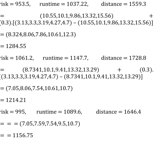
= (8.7341,9.43,9.41,11.74,13.29) + (0.3).

[(3.13,3.3,3.19,4.27,4.7) – (8.7341,9.43,9.41,11.74,13.29)] = (7.05,7.59,7.54,9.5,10.7)

(6)

216 risk = 953.5, runtime = 1037.22, distance = 1559.3

= (10.55,10.1,9.86,13.32,15.56) +

(0.3).[(3.13,3.3,3.19,4.27,4.7) – (10.55,10.1,9.86,13.32,15.56)] = (8.324,8.06,7.86,10.61,12.3)

= 1284.55

= (8.7341,10.1,9.41,13.32,13.29) + (0.3).

[(3.13,3.3,3.19,4.27,4.7) – (8.7341,10.1,9.41,13.32,13.29)]

= (7.05,8.06,7.54,10.61,10.7)

= 1214.21

risk = 995, runtime = 1089.6, distance = 1646.4

= = = (7.05,7.59,7.54,9.5,10.7)

= = 1156.75

So, this is clear that the best 2 solution are: , , then the solution is replaced by the new merged solution and give a best value better than .

Iteration 2

we have the best 2 solutions:

= (7.05,7.59,7.54,9.5,10.7), = 1156.75

= (7.05,8.06,7.54,10.61,10.7), = 1214.21

= (3.53,3.92,3.77,5.03,5.35)

Now: If = 0.3

= (7.05,7.59,7.54,9.5,10.7) + (0.3).

[(3.53,3.92,3.77,5.03,5.35) – (7.05,7.59,7.54,9.5,10.7)] = (5.99,6.49,6.41,8.16,9.1)

= 987.8

= (7.05,8.06,7.54,10.61,10.7) + (0.3). [

(3.53,3.92,3.77,5.03,5.35) – (7.05,8.06,7.54,10.61,10.7)]

= (5.99,6.82,6.41,8.94,9.1)

= 1028.2

risk = 843, runtime = 922.6, distance = 1393.4

When the solutions are compared in iterations 1,2 we find in iteration 1 is the best, then the optimal solution is: = = = (5.99,6.49,6.41,8.16,9.1), and the optimal value is: = = 987.8, with risk =813.8 threats, runtime = 885.8 ms, distance = 1332.2 m, also we can be found the coordinates as previous.

7 SYSTEM

A system of Microsoft Visual Basic for Applications (VBA) is designed and coded for testing the problem and is carried out on a computer with intel core i5 2.5 GHz CPU and 4 GB of ram, so it is some images describe the design of this system:

Firstly, the Evolutionary Optimization is used with BB-BC, Secondly, it is used with PIO technique.

7.1 Test 1 Evolutionary Optimization with BB-BC Now, the evolutionary optimization technique is used to build a new merged solution by using the crossover of components in the best solutions which be obtained from using the BB-BC technique only and the results as follows:

No of iterations = 3, α = 1 and rand = 0.2

Fig. 4 The final results with No of iterations = 3

The next chart shows the changes of objective functions over number of Iterations Changes at α = 1, rand = 0.2:

Fig. 9 Changing the objective functions values over number of iterations changes at α = 1, rand = 0.2 in bb-bc with evolutionary optimization technique

Comparing the results of test 1 in [2] and current test we note that at iteration 3 the results of using BB-BC technique only is better than the using of evolutionary with BB-BC, but BB-BC with Evolutionary reached to the optimal

(7)

BB-BC with Evolutionary Optimization the solution reached the optimal state at iteration 2 directly, since using the BB-BC only reached to the optimal state at best value of α in iteration 4 as follows:

Fig. 10 The final results at best values of α using bb-bc with evolutionary optimization reached the optimal state at iteration 2 directly

Now, we will use the Evolutionary Optimization with PIO technique.

7.2 Test 2 Evolutionary Optimization with PIO

Now, the evolutionary optimization is used to build a new merged solution by using the crossover in the components of the new solution and applying the PIO technique to get the new optimal solution, and run it in the system at different values of number of iterations Nc1 and Nc2, with these inputs R = 0.2, rand = 0.3, Nc1 = 3 and Nc2 = 1, as follows:

Fig. 11 The new merged solution excludes one of the best solutions

Here we note that the new merged solution can excludes one of the best solutions.

Fig. 12 The final results at Nc1 = 3 and Nc2 = 1

At Nc1 = 30 and Nc2 = 1

At Nc1 = 179 and Nc2 = 1

At Nc1 = 3000 and Nc2 = 1

At Nc1 = 100000 and Nc2 = 1

The next chart shows the changes of objective functions over number of iterations:

Fig. 15 PIO with evolutionary optimization

Comparing the current results with these in test 2 in (Ahmed, 2018) we deduce that the evolutionary optimization can improve the optimal values which gives best convergence to the optimal state.

Now, we can get the coordinates of the new IT units’ locations from the law of distance between 2 points:

(26)

considering the datacenter coordinates at (0,0).

8 CONCLUSION

Observing the results, we can deduce that the addition of evolutionary optimization to BB-BC technique don’t give the best result but it can reach to the optimality in more fast behavior than the state of using the BB-BC only in solving the problem under study, since in the state of using the evolutionary optimization with the PIO technique we can obtain the best convergence to the optimal state in results and time.

ACKNOWLEDGEMENTS

We would like to express our sincere thanks to the team of Digital Information Network in Benha University who provided me with all statistics and research facilities. Without they precious support it would not be possible to conduct this research.

RECOMMENDATIONS

A parameter analysis study is recommended for the different used metaheuristic techniques to obtain the best values of these parameters which lead to the optimal state directly, also, a new hybrid approach can be built for solving the problem under study consists of the most efficient techniques with comparison study is achieved between the new results and the other obtained in this paper.

REFERENCES

[1] Ack, T., Hammel, U., & Schwefel, H., “Evolutionary computation Comments on the history and current state,” IEEE Transactions on Evolutionary Computation, vol. 1, pp. 3–17, 1997.

[2] Ahmed, A. A. Zakzouk, Mohamed, S. A. Osman, Ramadan, A. Zeaneddin, & Hamdeen, A. Khalifa, “Solving the Multi-objective Facility Location Problem Using Big Bang Big Crunch and Pigeon Inspired Optimization Techniques,” American Scientific Research Journal for Engineering Technology and Sciences, vol.50, pp. 1-21, 2018.

[3] Ajith, A., Lakhmi, J., & Robert, G, Evolutionary Multi-Objective Optimization. USA, Springer-Verlag London Limited, 2005.

[4] Branke, J., Deb, K., & Miettinen, K., Multi-objective optimization interactive and evolutionary approaches. Germany, Springer-Verlag Berlin Heidelberg, 2008.

(8)

218

Intelligent Computing and Cybernetics, vol. 7, pp. 24-37, 2014.

[6] Hiba, Bederina, & Mhand, Hifi, “A hybrid multi-objective evolutionary optimization approach for the robust vehicle routing problem,” Applied Soft Computing, vol. 71, pp. 980-993, 2018.

[7] Irina, H., Christine, L., Mumford, B., & Mohamed, M. Naim, “A hybrid multi-objective approach to capacitated facility location with flexible store allocation for green logistics modeling,” Transportation Research Part E, vol. 66, pp. 1–22, 2014.

[8] Kalyanmoy, Deb, Multi-Objective Optimization Using Evolutionary Algorithms. USA, John Wiley & Sons, 2001.

[9] Matias, P., Germán, R., Nesmachnow, S., Ana, C., “Multi-objective evolutionary optimization of traffic flow and pollution in Montevideo,” Applied Soft Computing, vol. 70, pp. 472-485, 2018.

[10] Nesmachnow, S., “An overview of metaheuristics: accurate and efficient methods for optimization,” International Journal of Metaheuristic, vol. 3, pp. 320–347, 2014.

[11] Osman, K., & Eksin, I., “A new optimization method: big bang- big crunch,” Advances in Engineering Software Journal, vol. 37, pp. 106–111, 2006.